深度学习

吴恩达深度学习课程
第一课 — 神经网络与深度学习： av66314465
第二课 — 改善深层神经网络：超参数调试、正则化以及优化：av66524657
第三课 — 结构化机器学习项目：av66644404
第四课 — 卷积神经网络：av66646276
第五课 — 序列模型：av66647398

专业课概述

AlphaGo使用的机器学习内容：蒙特卡洛树搜索，两个深度神经网络

• 神经网络内容：
  • 卷积神经网络：ImageNet（残差网络），Inception
    • 实际应用：目标检测，人脸验证，图片风格转换
  • 序列模型：网络结构，GRU，LSTM
    • 实际应用：词嵌入，语言模型，注意力机制，触发语检测
• 神经网络使用领域：
  • 计算机视觉
    • 实际运用
      • 图像分类
      • 语义分割
      • 物体识别和检测
      • 运动和跟踪
      • 视觉问答
      • 三维重建
  • 自然语言处理
    • 主要是由两个内容组成
      • 自然语言理解
      • 自然语言生成
    • 实际运用
      • 语音识别
      • 机器翻译
      • 语音合成
      • 人机对话
      • 语音助手
      • 问答系统
      • 机器阅读
  • 生成对抗网络
    • 特质
      • 通过训练数据进行生成需要的数据
      • 属于监督学习方法
      • 同时训练一个生成网络和一个判别网络
        • 生成网络：生成逼真的图片欺骗判别网络
        • 判别网络：区分生成图片和真实图片
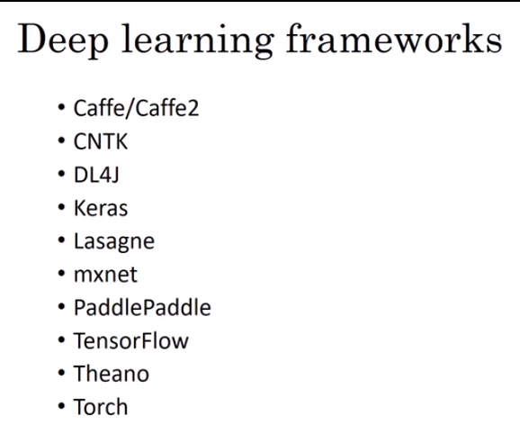
• 深度学习框架
  • TensorFlow from Google for Industry
    • 19.10 -> Version 2.0
    • 专业课主要学习的框架，学习版本为1.x，2.0版本与1.x版本差别很大，需要分开学习
      • 编程语言：python 3.x
      • 编程环境：Anaconda, Jupyter Notebook, TensorFlow 1.x
  • Keras into TensorFlow
  • Pytorch use Python from Facebook for study
  • PaddlePaddle from Baidu
  • Deeplearning4j use JAVA
  • Mxnet from Amazon
  • Caffe&Caffe2 into Pytorch
  • CNTK from Microsoft
  • Theano is ancient
  • Chainer use Python
• 学习辅用网上视频课：吴恩达深度学习课程

第一课：视频课1-6 导论

1. 学习顺序

   1. (周1-4)Neural Networks and Deep Learning
      • Cats Recognition
   2. Improving Deep Neural Network: Hyperparameter tuning(参数调整) , Regularization(正则化) and Optimization(优化)
   3. Structing(结构化) your Machine Learning project.
   4. Convolutional Neural Networks 卷积神经网络
   5. Natural Language Processing.

2. What is a neural network?

   A function to estimate a result which need a lot of data of parameter to confirm how is the final result decided.

   We do not setting the method detail of solving problem

3. Supervised Learning 监管学习

   Give a series of Input and Gain a series of Output.

   • Example:

     ​ Home features -> Price (Standard NN)

     ​ Ad, user Info … -> Click on ad? (Standard NN)

     ​ Image -> Objects (CNN)

     ​ Audio -> Text transcript (RNN【Recurrent Neural Network】)

     ​ English -> Chinese (RNN)

     ​ Image, Radar Info -> Position of other cars. (Custom / Hybrid)

   Standard NN 标准神经网络，Convolutional NN 卷积神经网络，Recurrent NN 循环神经网络

   Neural Network Make Computer more easy to understand unstructured data.

4. Why are they just now taking off?

   scale of data and computation is growing rapidly, and the progress in algorithms.

   Using a new way (ReLu function instead of Sigmoid function) to faster the speed of training a model.

   

第一课：视频课7-24

7. Binary Classification
   • A great algorithm to process the entire train sets with a great speed.
   • A introduction of forward pass or forward propagation step and backward pass or backward propagation step 前向传播和反向传播
   • Logistic regression 逻辑回归
     • An algorithm for binary classification.
   • Important Notation
     • ‘n’ is the length of height of the matric X, ‘m’ is the count of training examples (or looks like { (x1, y1) … (x(m), y(m) ) } ).
     • there are two sets, one of them for train, another for test.
     • (Xn, Y) is a specific vector.
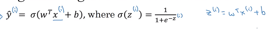
8. Logistic Regression
   • Given x, want y hat or y^.
   • Parameters: w (matrix), b (real number)
   • Output: y^ = w^T * x + b (Sigmoid function) = Sigmoid(Z)
     • 
     • 
     • learn about w and b to know how y become a good estimate.
     • 
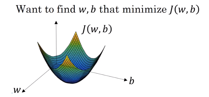
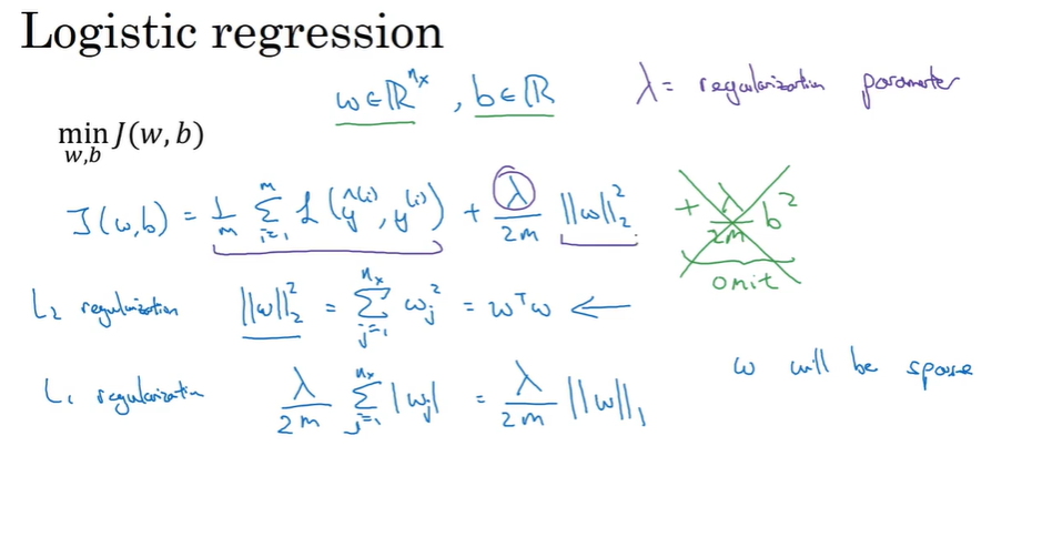
9. Logistic Regression cost function

To train the parameters W and B of the logistic regression model, We need to define a cost function

To get the best prediction, we want the y Hat can be more and more near to the i-th example.

Lost funcion is used to measure how well our algorithm is doing.

Here is the not good algorithm: (which will get serveral global optimums.)


Here is the better algorithm: (of which graph is convex)


Cost function: the cost of the parameters.


Compute the total cost of the whole sets, Measure how well the performance of your trained model.

10. Gradient Descent 梯度下降法

The method to train the w and b.

ways: Find the minimum or to say the global optimum.

The real usage of Gradient Descent.

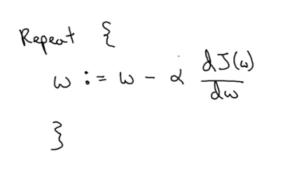
Parameters in this function:

​ α ：learning rate ：which to control how big a step we take on each iteration or gradient descent.

​ w := means updated w equal to the right

The Key of function

• using derivatives导数 to find the side which is more near to the optimum
• and update the nearest value and repeat it until you can not fould the next value.

11. derivatives 导数

略（PS:作为一个正在考研的人，要是这里还需要这种入门级的教学，我就别考了hhh）

13. Computation Graph 计算图

Also the introduction about derivaives, but the graph makes the procedure of whole computation a lot easier to be comprehended.

Example:

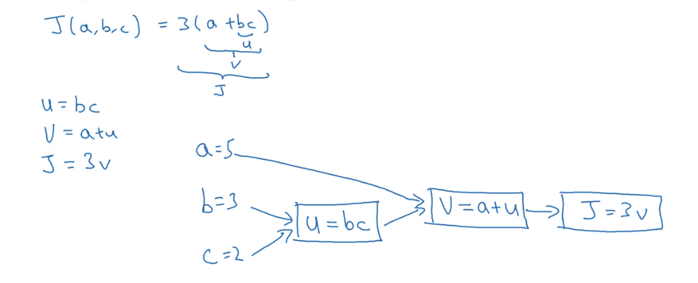
The Compute of Derivatives in Computation Graph


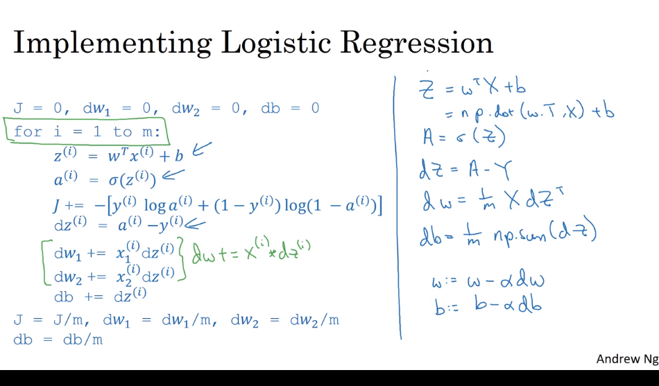
15. Logistic Regression - Gradient descent 逻辑回归中的梯度下降法

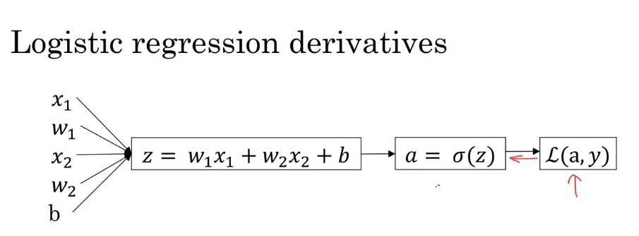
And Find the derivatives for L :

da = dL / da = - y / a + (1 - y) / (1 - a)

dz = dL / dz = dL / da * da / dz = dL / da * a(1-a) = a - y

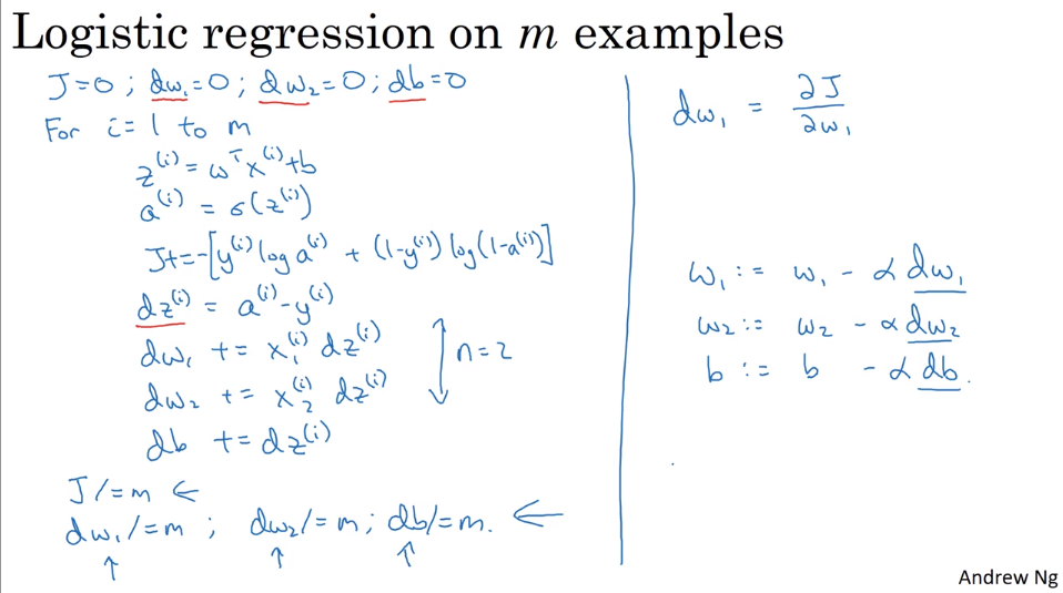
**dw1 = dL / dw1 = x1 * dz = x1 * (a - y) **

**dw2 = x2 * dz **

db = dz

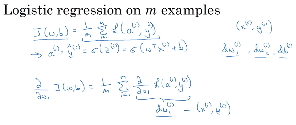
using Gradient descent on M samples

The used function is J(w, b)

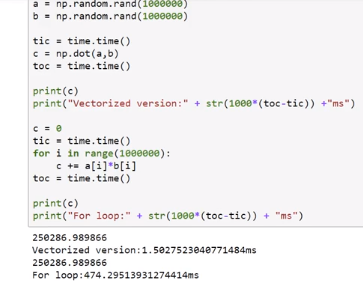
17. Vetorization 向量化

A great important method to forbid repeatitive and inefficient looping

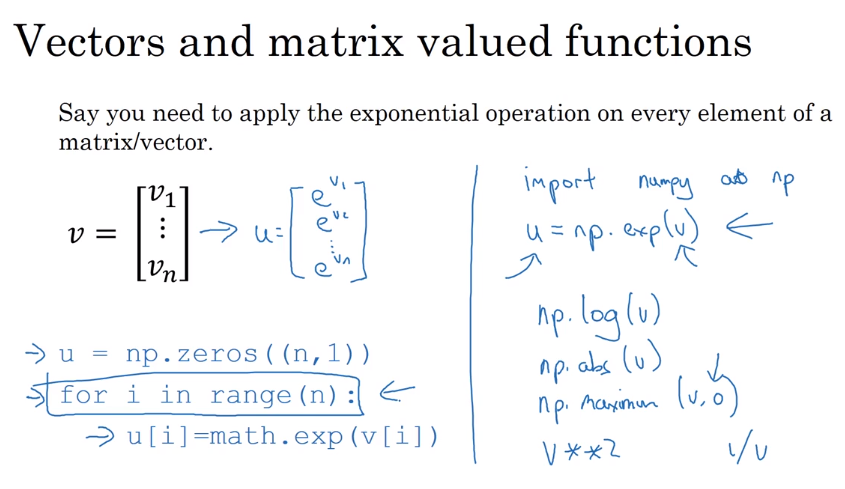
19. Vectorizing Logistic Regression 向量化逻辑回归

Using Python Module – Numpy to Simplify the Code

20. Vectorizing Logistic Regresion’s Gradient Computation 向量化逻辑回归的梯度计算

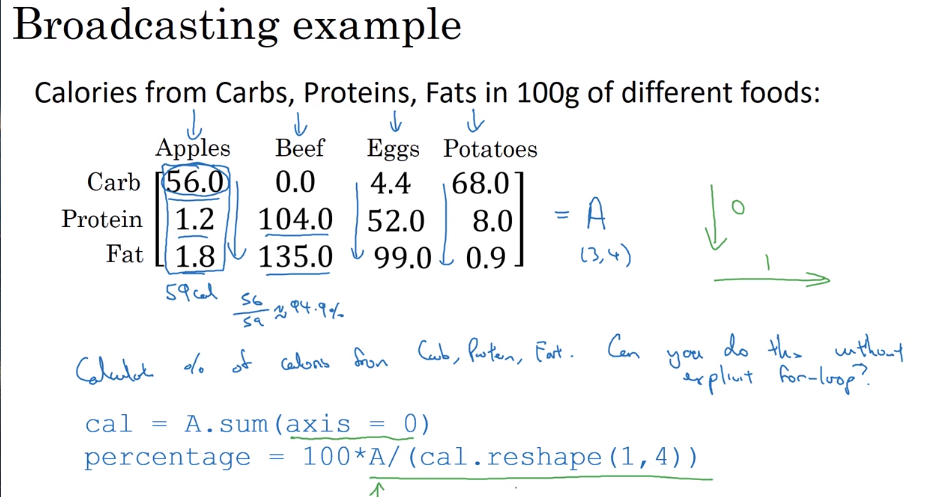
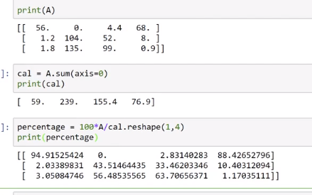
21. Broadcasting in Python

第一课：视频课25-35

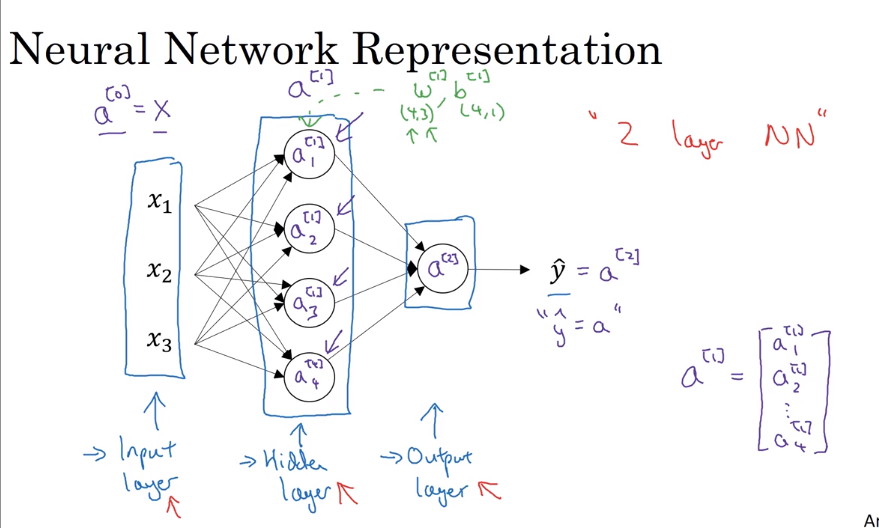
25. Neural Network Overview

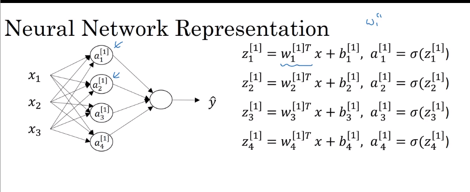
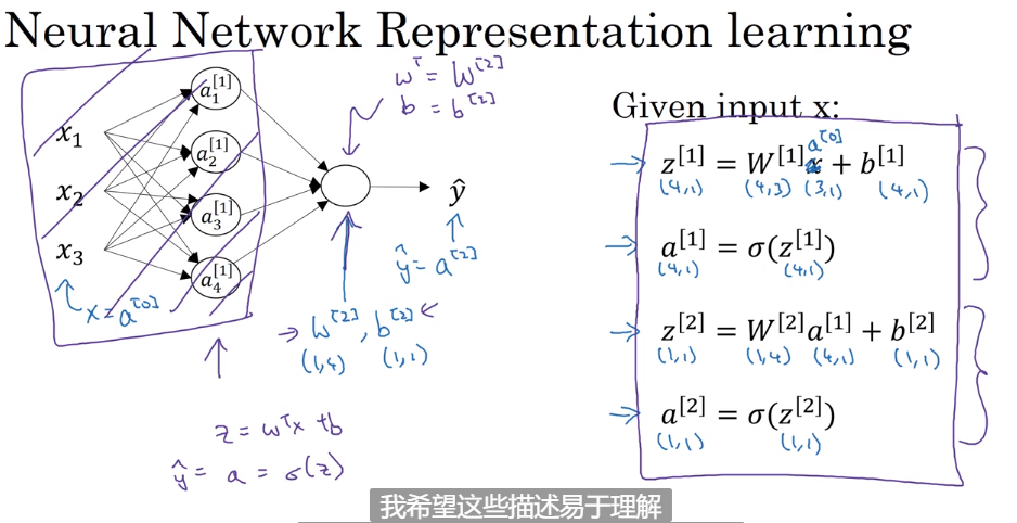
26. Neural Network Representation

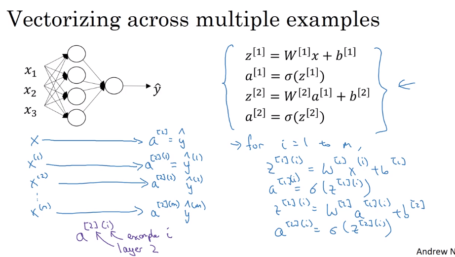
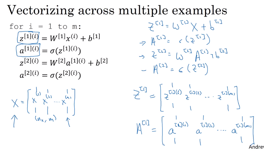
28. Vertorizing

30. Activation functions

Here are four useful and often activation function:

• sigmoid : It doesn’t to be used any more, because it has some disadventages
• tanh: limit the output between 0 and 1
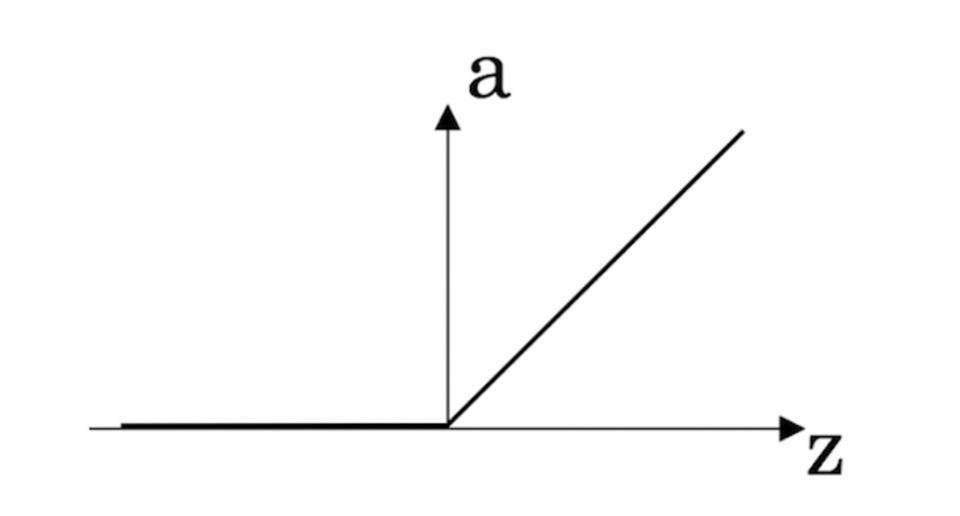
• ReLU: Rectified limit Unit – a = max(0, 1) (Mr.Wu recommend)
• Leaky ReLU: Rectified limit Unit which is not zero when input go down zero.

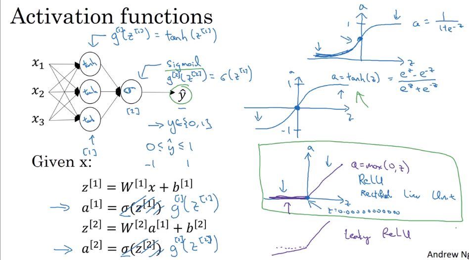
31. Why we use non-linear activate function.

If we use linear activate function in neural network, the whole hidden layers is useless, and it may be OK when you wanna computing output a real number.**So we only use linear function in the final output layer, except for some special circumstance. **but In that case, using ReLU is fine, too

32. the deriviatives of Activate functions

• sigmoid -> a’ = sigmoid’(z) = a (1 - a)
• tanh -> a’ = tanh’(z) = 1 - a^2
• ReLU -> a’ = (max(0, z))’ = 0, if z < 0; 1, if z >= 0.
• Leaky ReLU -> a’ = (max(0.01 * z, z))’ = 0.01, if z < 0; 1 if z >=0.

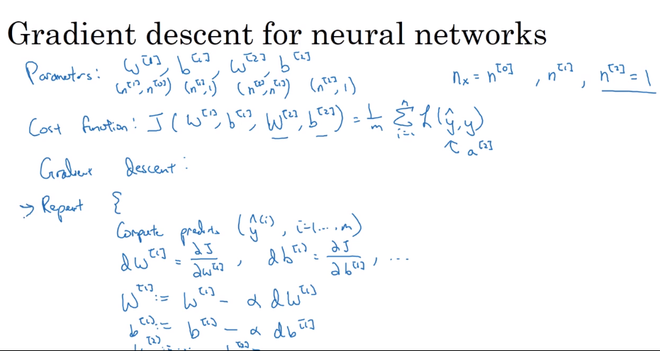
33. Gradient descent for neural networks

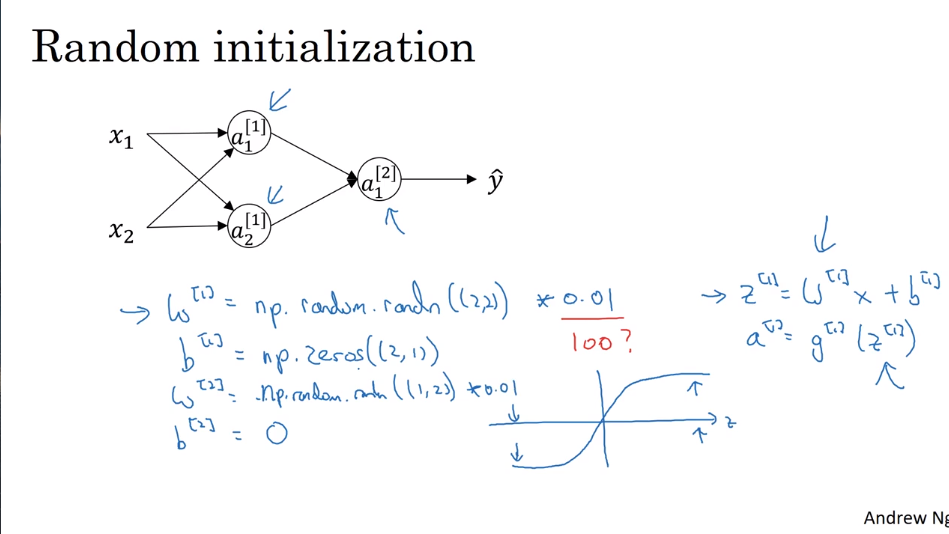
35. Randomly Initialization

If we don’t randomly initialize paremeter W, we will get the same result from each unit in one

layer. It will make out gradient descent to doesn’t work by makes the units output the same results.

b initialized by zeros is OK, but W should be randomly initialized.

In Python:

• w1 = np.random.rand((a, b)) * 0.01 (why here is 0.01 instead of 100 or 1000?)

  • the latter multiplier usually be very small because if this parameter become too large, it makes the sigmoid function or tanh or others useless, hence it makes the learning too slow.

• b1 = np.zero((b, 1))

第一课：视频课36-43

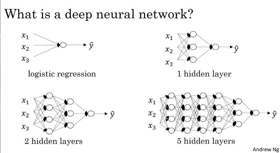
36. Deep L-layer Neural network

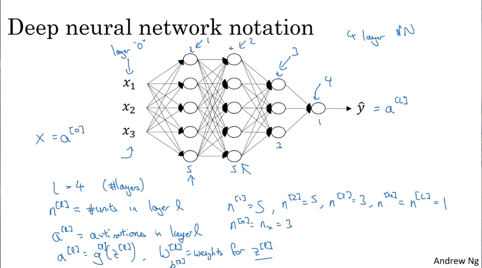
38. getting your matrix dimensions right

单变量的情况下：

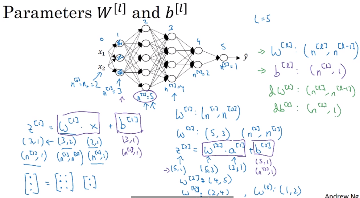
Z[l] -> (n[l], 1); A[I] -> (n[l], 1);

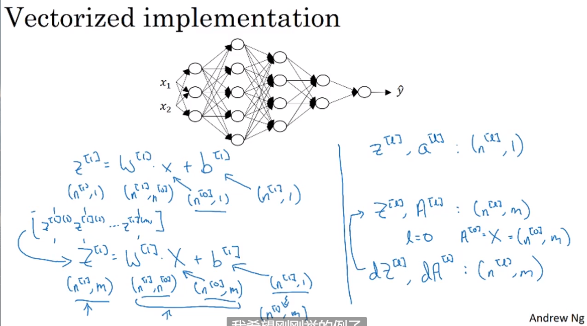
向量化后：when function plus parameter b, python will automatically using broadcast to duplicate b into a (n, m) matrix

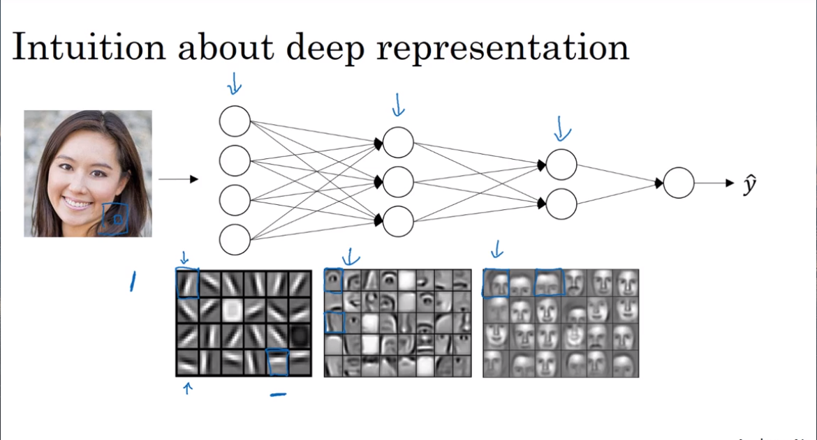
39. Why deep representations?

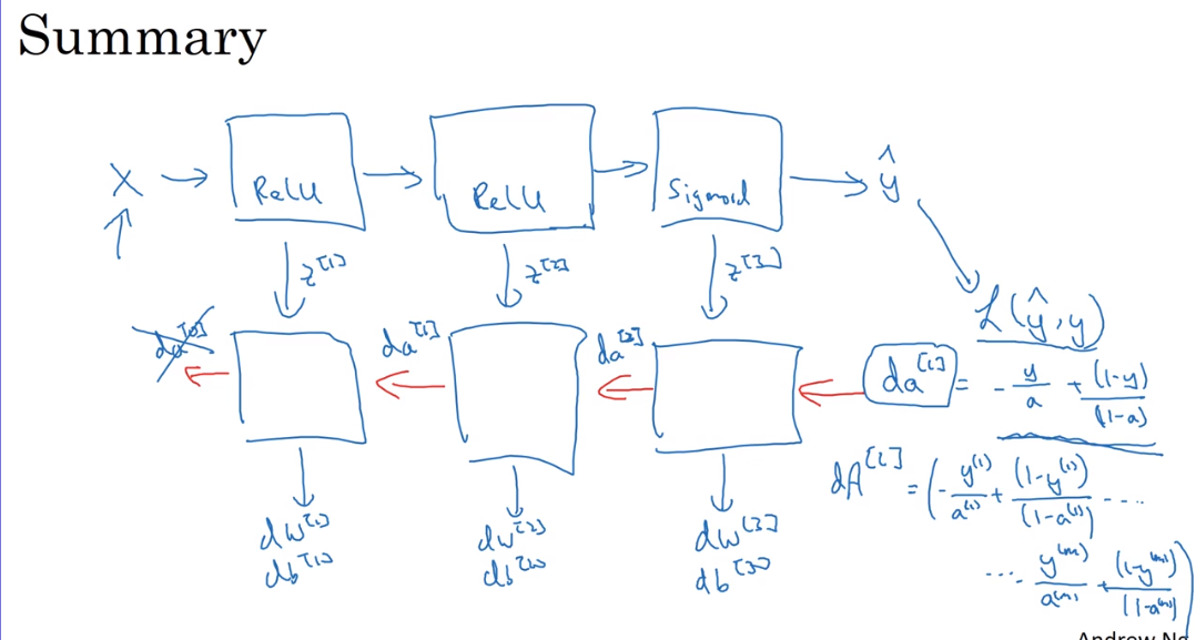
40. Building blocks of deep neural networks

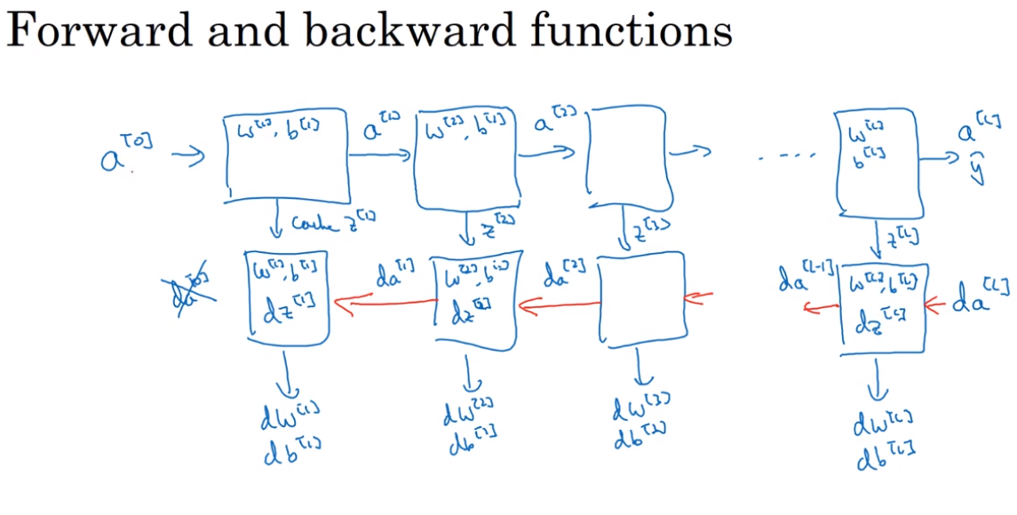
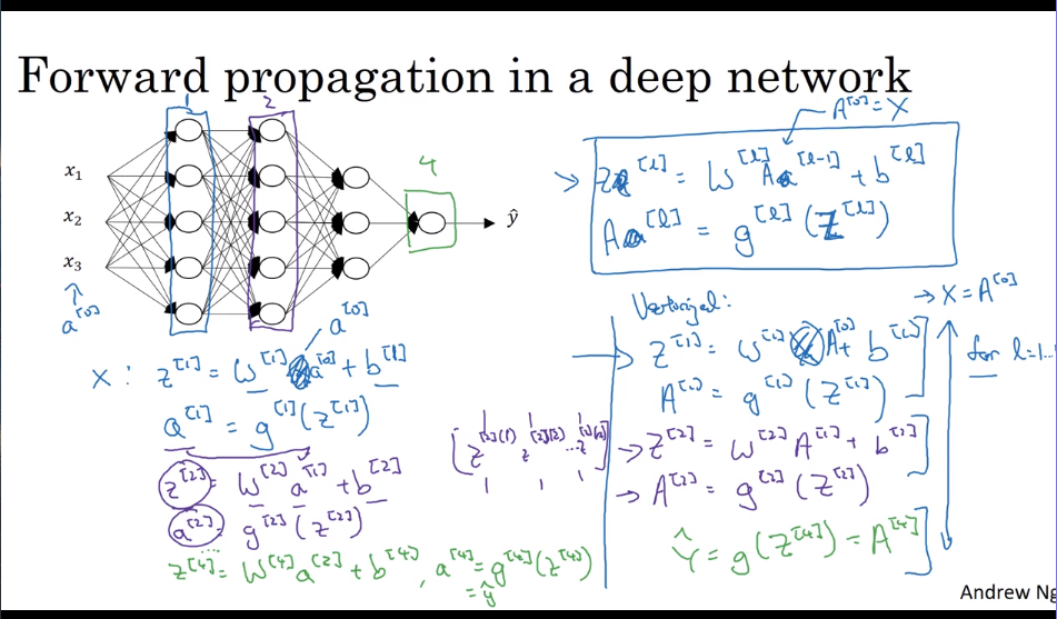
37. Forward propagation in a deep network

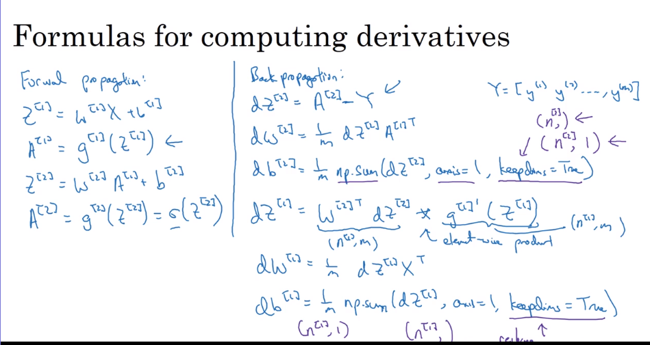
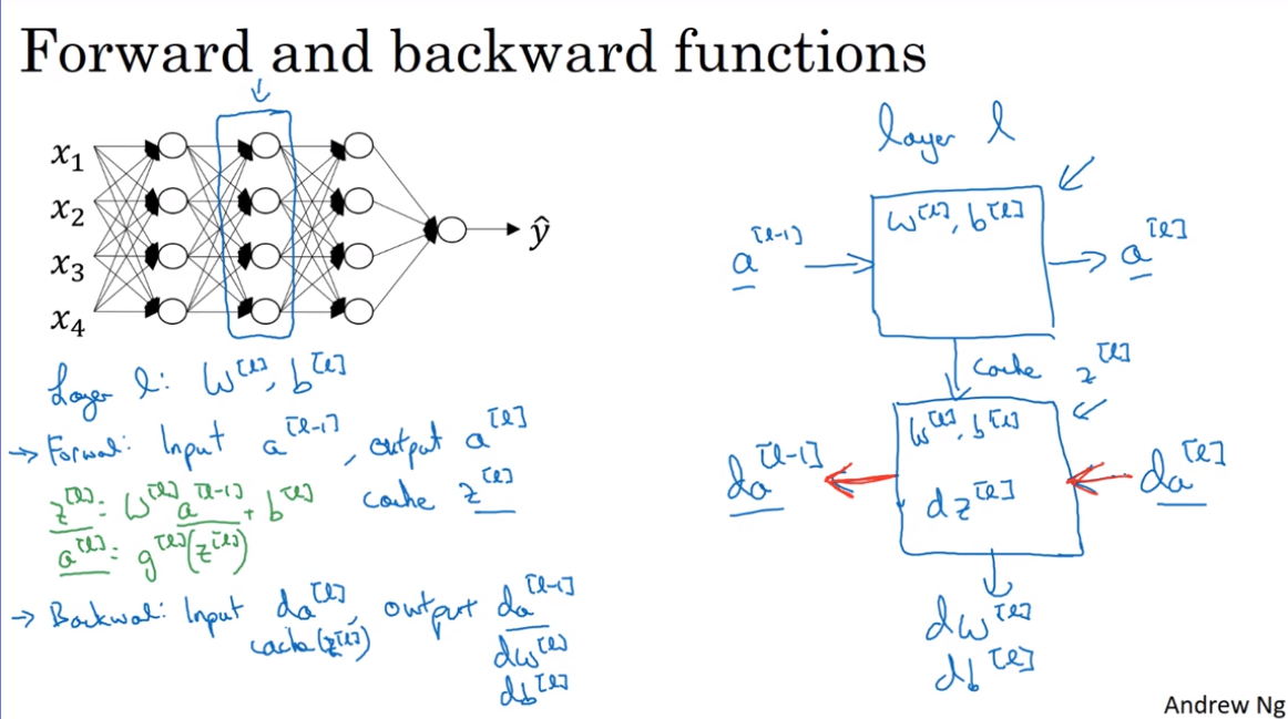
41. Forward and backward propagation

Forward propagation:

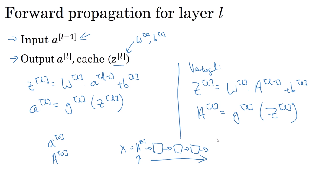
Backward propagation:

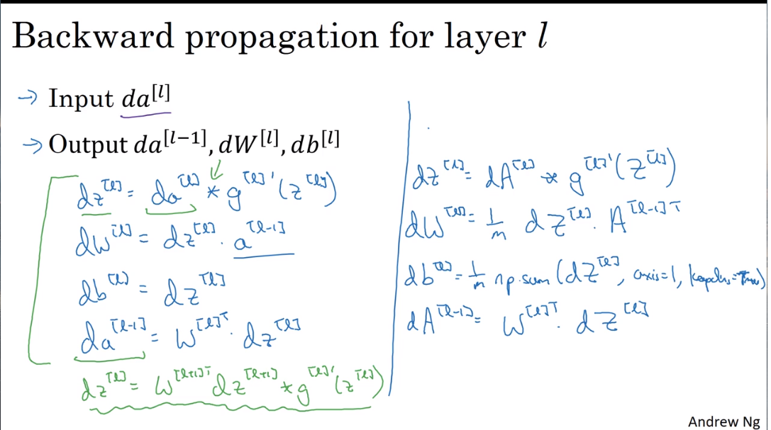
Noticing the backward propagation initialization parameter ==dA==

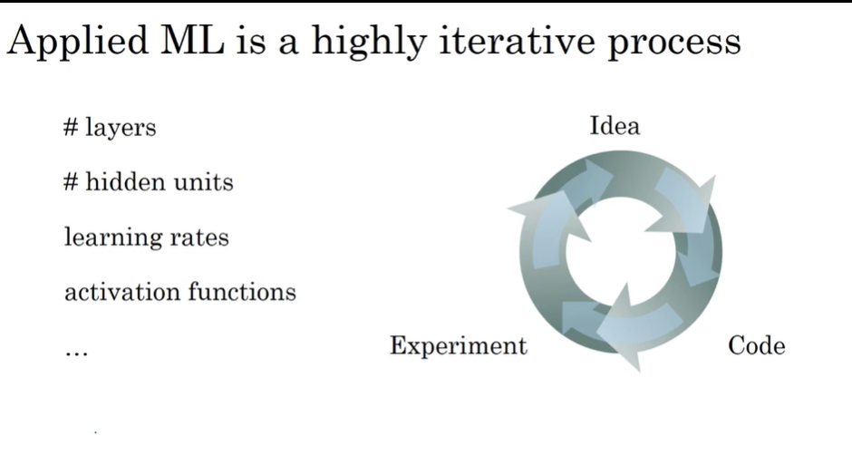
42. Parameters ==vs== Hyperparameters

Hyperparameters is controlled by researchers, which could directly effect the paramters ==W, B==;

第二课：视频课1-14

1. Train / dev / test sets

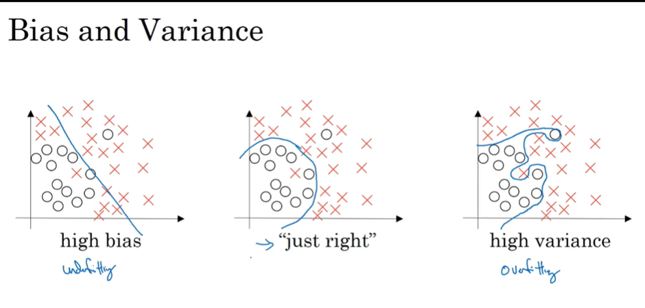
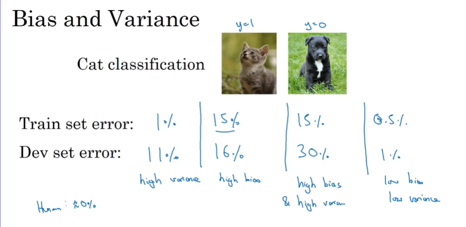
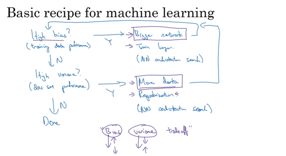
2. Bias / Variance 偏差/方差

3. Basic recipe for machine learning

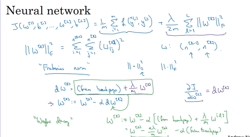
4. Regularization 正则化

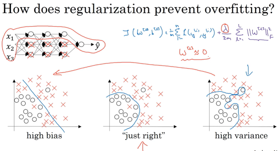
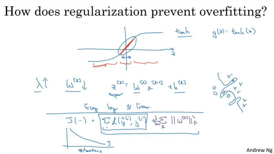
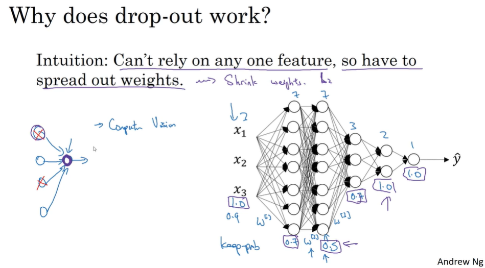
5. Why regularization reduces overfittings?

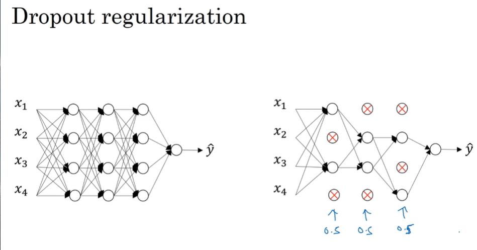
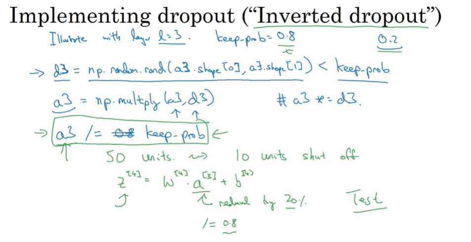
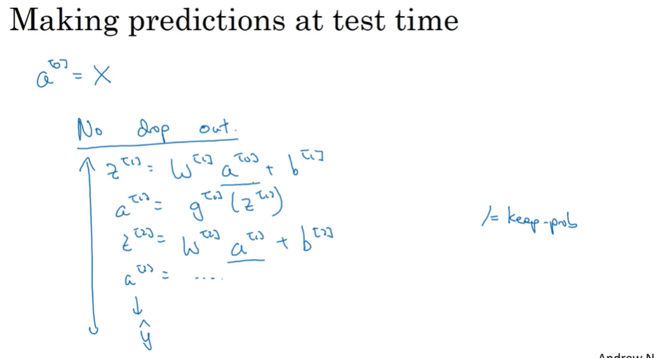
6. Dropout regularization 随机失活正则化

Randomly choose several units in each layer and set them disabled

8. Other regularization methods

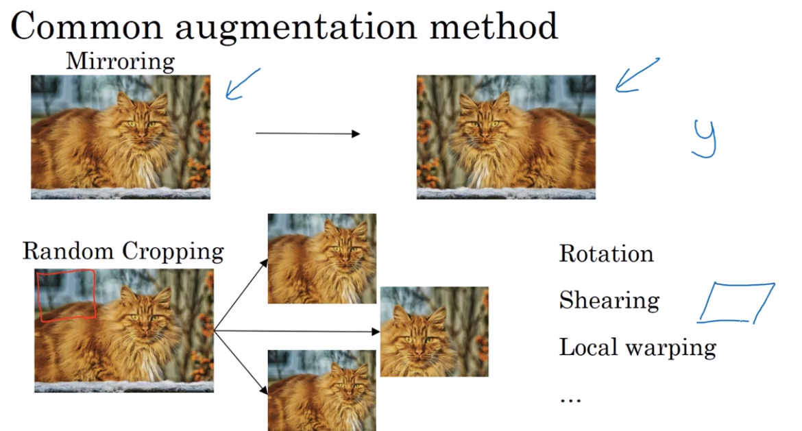
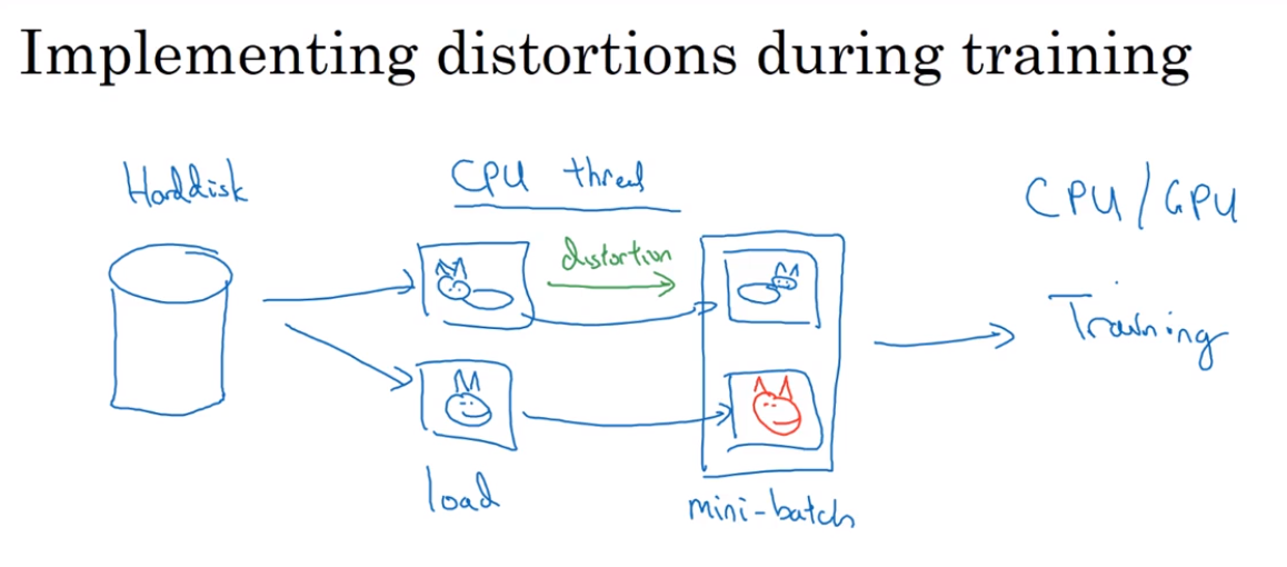
Data augmentation (when we can’t get more data)

flipping horizontally, rotated or distortion

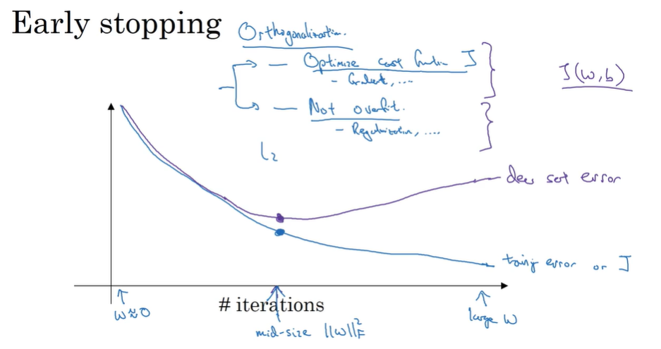
Early stopping (avoid overfitting)

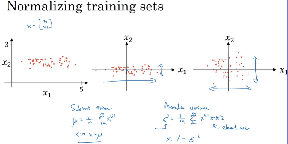
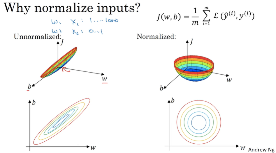
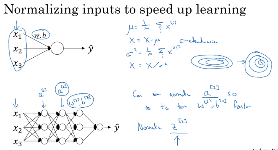
9. Normalizing inputs

There are two steps:

• subtract mean (zero mean)
• normalize variance

Use the same mu and sigma in train set and test set

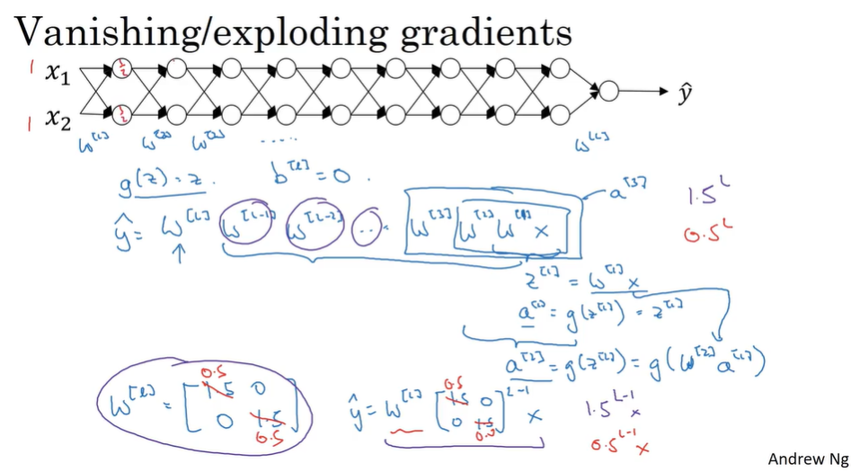
10. Vanishing / exploding gradients

If each W greater than 1, the activation will be exploding.

If each W smaller than 1, the activation will be vanishing.

They will also make the learning very slow.

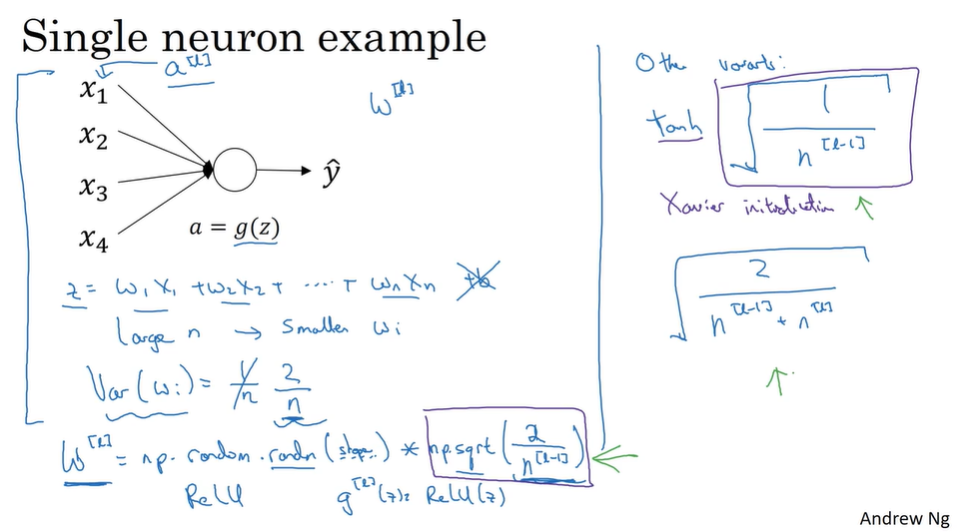
11. Weight initialization for deep network

Because of the existence of Vanishing / exploding gradients, we have to take careful in weight initialization.

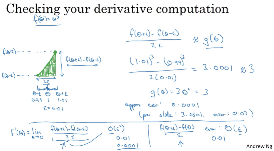
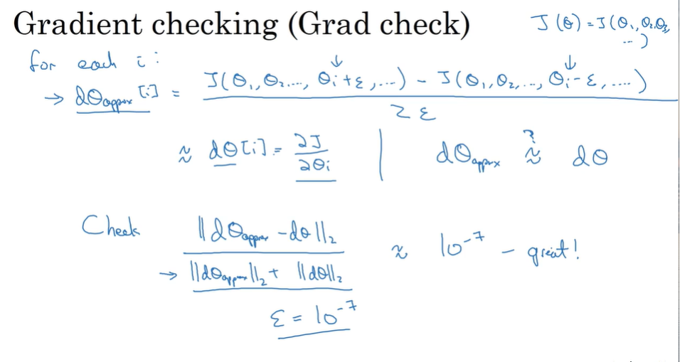
12. Gradient checking

For checking if the compute of derivatives is correct.

Numerical approximation of gradients 梯度数值逼近

Using the double sides derivative, which makes the Error much less than one side derivative.

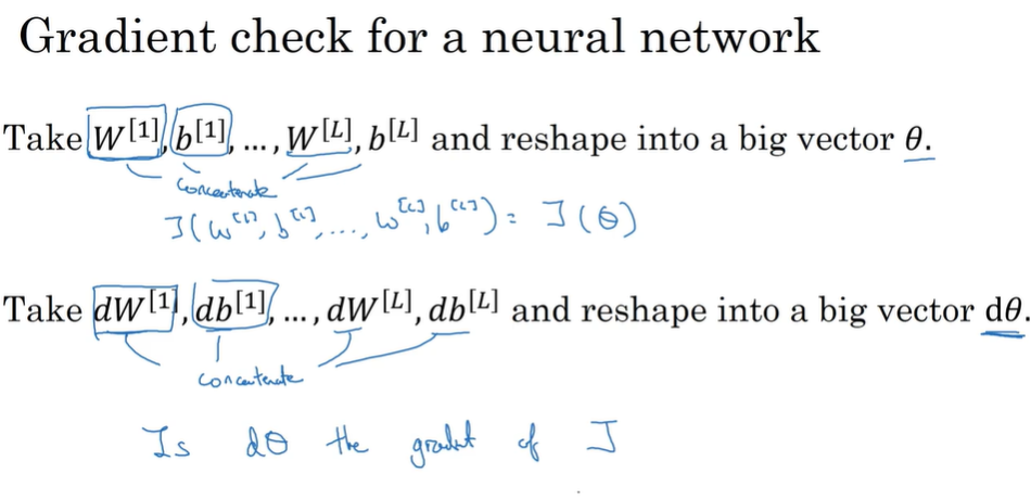
Gradient checking

14. Gradient Checking implementation notes.

• Don’t use in training, only to debug.
• If algorithm fails grad check, look at components to try to identify bug.
• Remember regularization.
• Doesn’t work with dropout.
• Run at ramdom initialization; perhaps again after some training.

第二课：视频课15-24

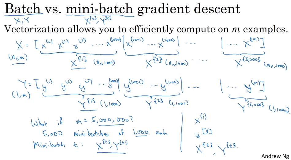
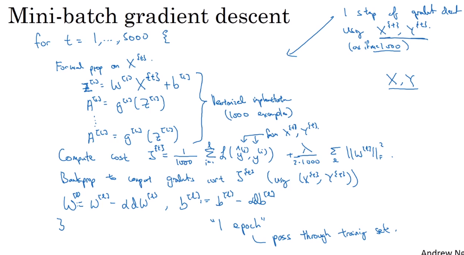
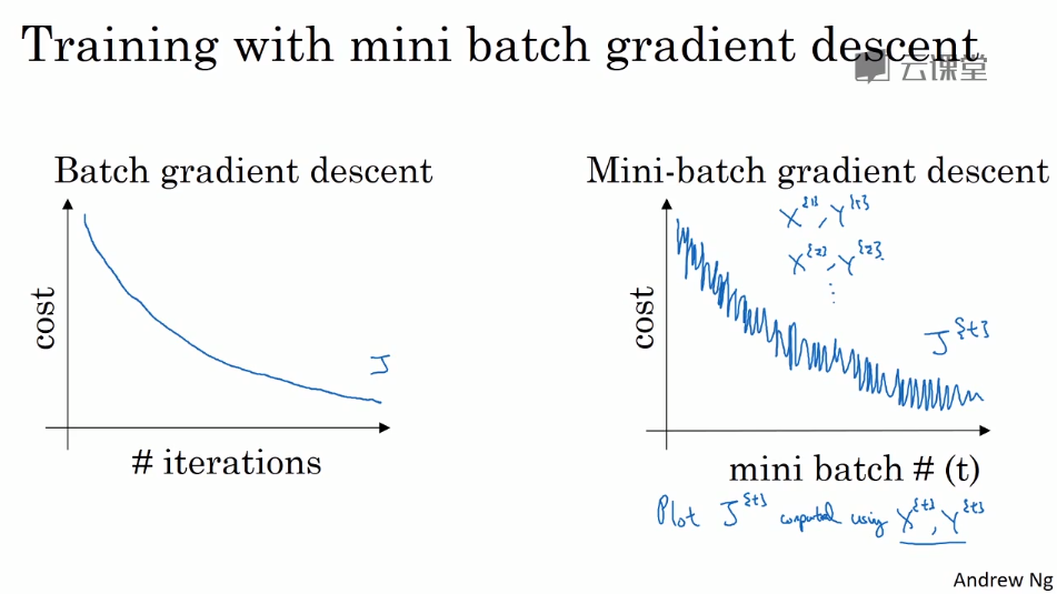
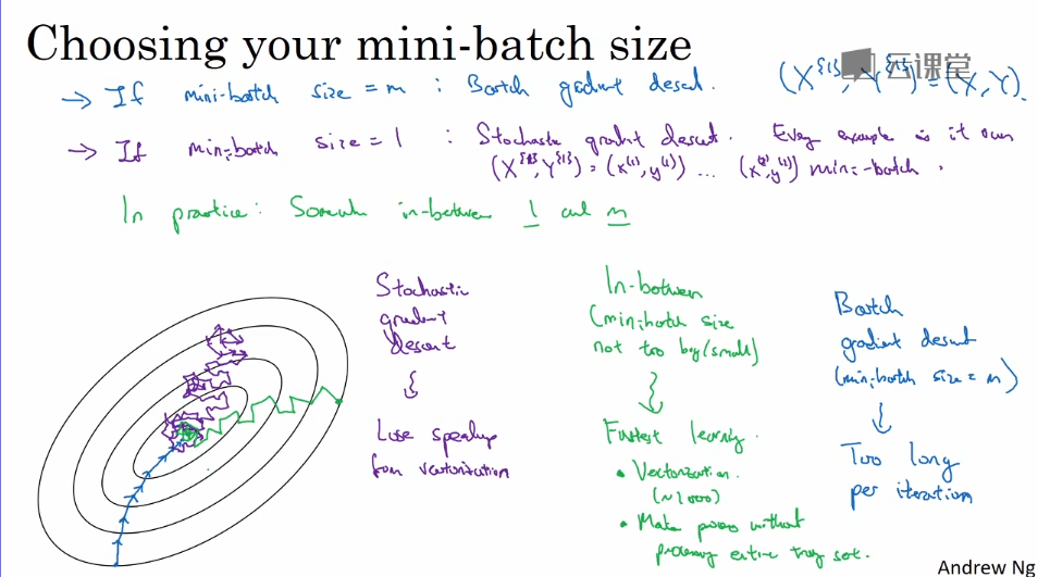
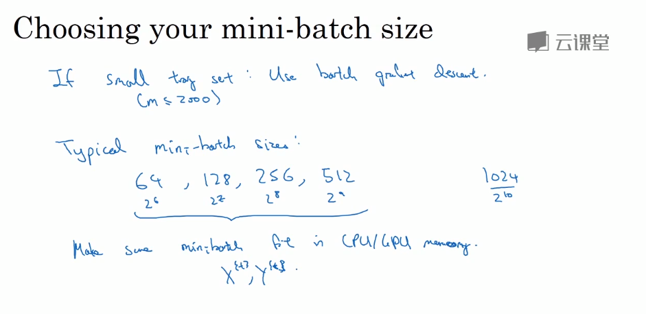
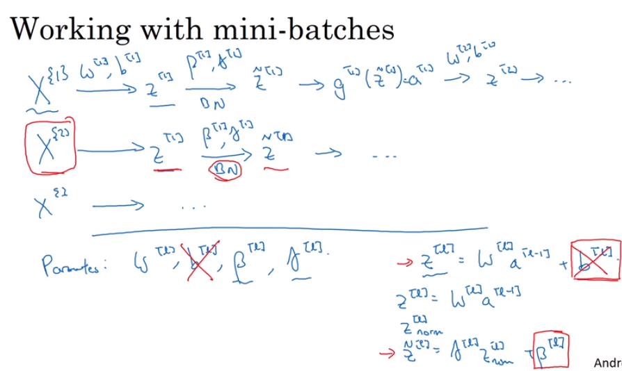
15. Mini-batch gradent descent

When the count of sample is too large, the speed of using your algorithm will still be too slow to compute.

Mini-batch means a little sets of trainning samples extracted from a whole tremendous training samples sets.

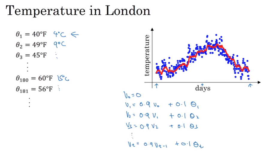
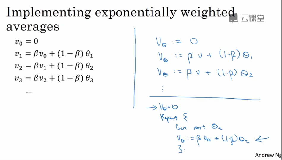
17. Exponentially weighted averages. 指数加权平衡

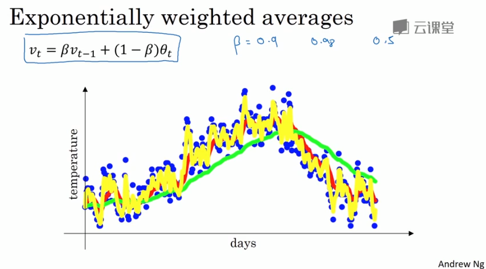
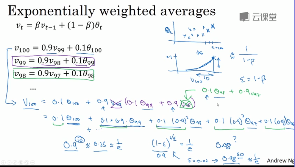
The adventages of exponentially weighted averages:

• it just takes up one line of code basically. 只占用一行代码
• and just storage and memory for a single row number to compute this exponentially weighted average. 只需要存储单行数字内容
• not the best and most accurate way to compute average.

19. Bias correction in exponentially weighted averages

In last example, using exponentially weighted averages might make the first several averages too low to be accurate to portray the first several days temperature.

So, we have to use bias to fix it.

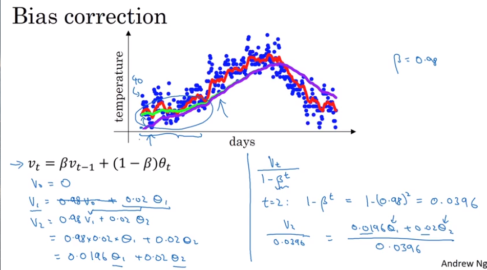
The bias will go very near to zero when days go up, so we don’t worry about the influence of bias in rear samples.

Most people don’t care about it unless you have to concentrate on the first several indics

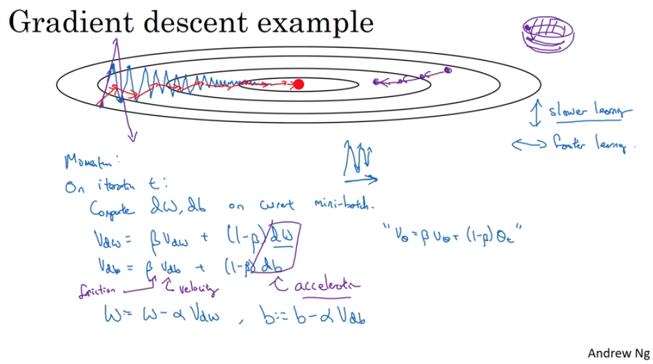
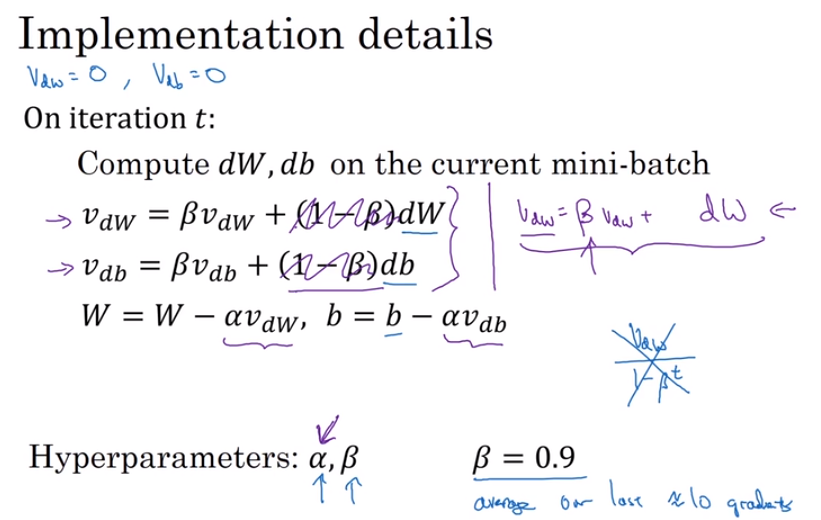
20. Gradient descent with momentum 动量梯度下降法

In previous methods, we have to make the learning rate low lest make the predictions go far away from the minimum.

In Gradient descent with momentum, we using the exponentially weighted averages as our forward momentum to keep the learning orientation is point to the position of the minimum.

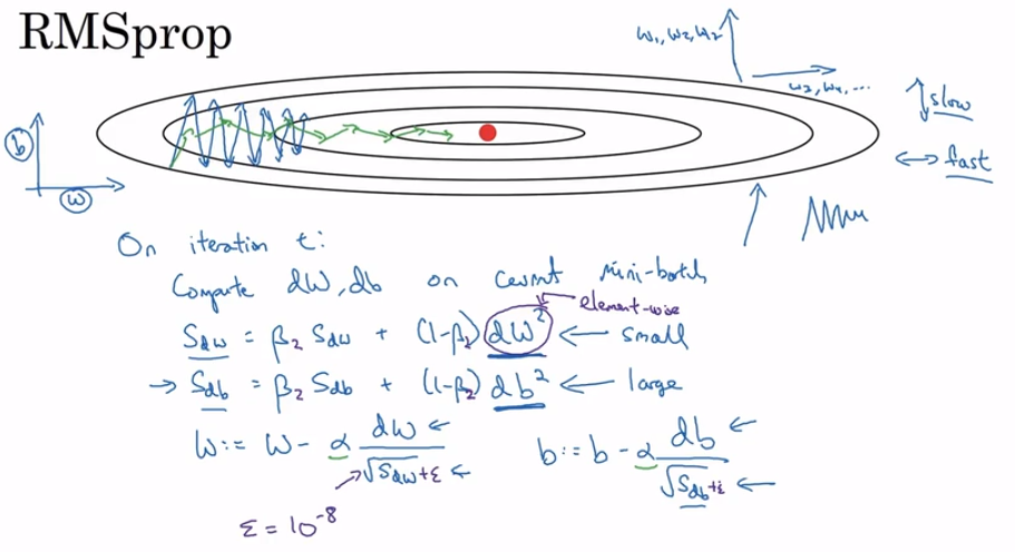
21. RMSprop

Another way to speed up gradient descent.

I do not really comprehend understand it.

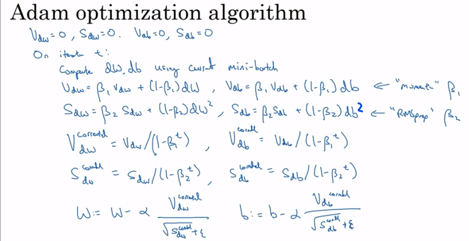
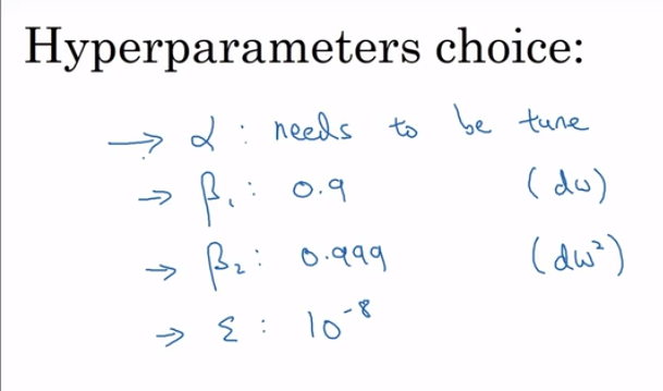
22. Adam optimization algorithm

Adam : Adaption Moment Estimation

Another way to speed up gradient descent using in generally

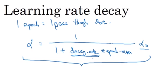
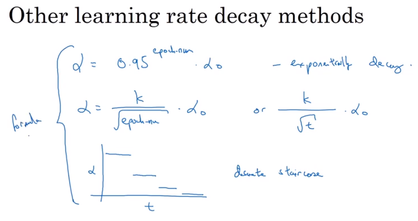
23. Learning rate decay

There are several way to make the learning rate goes down with the iteration goes through.

24. The problem of local optima 局部最优问题

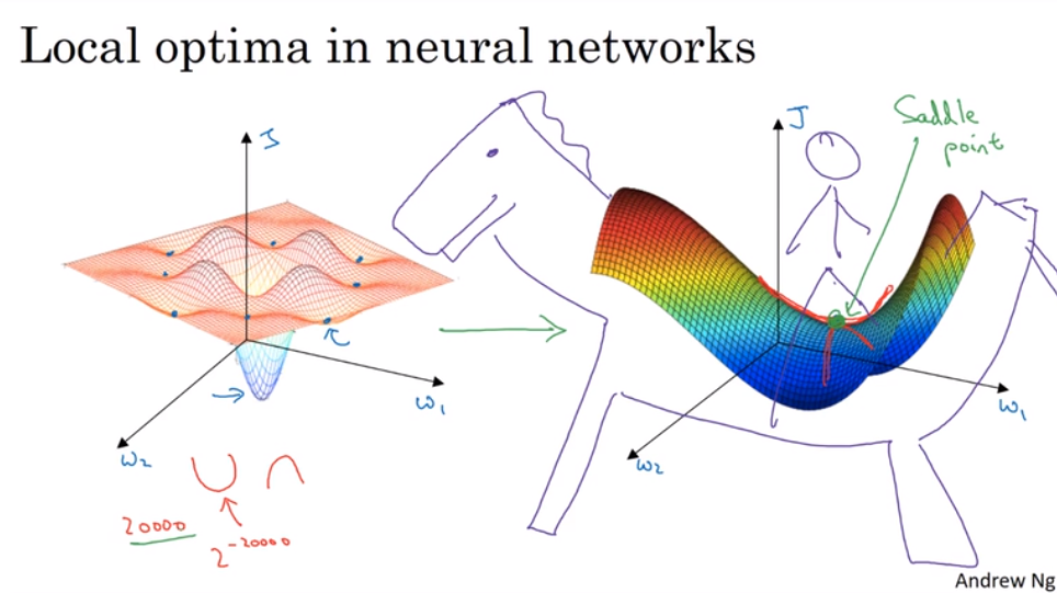
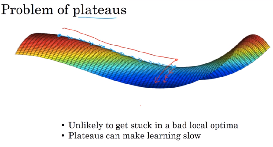
The optimization methods could help us exemplify from the local optima

第二课：视频课25-35

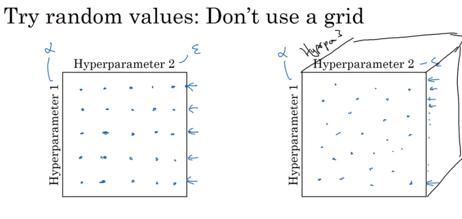
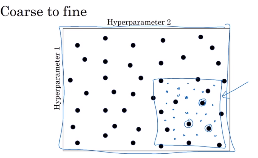
25. Tuning process 调试处理

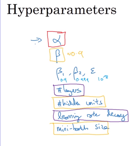
Find the best hyperparameters‘ values

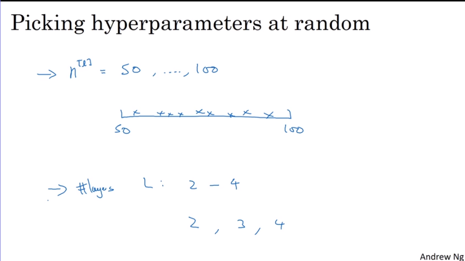
26. Using an appropriate scale to pick hyperparameters

A normal way to choose but not for all.

A special way for estimate the hyperparameters which is sensitive for a very small changes.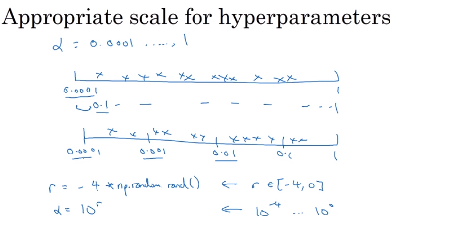

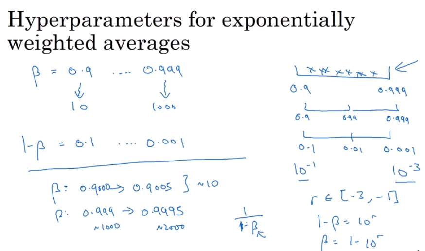
Because of the trait of exponentially weighted averages, which is when it comes too close to 1, the influence of it will become more and more intensive.

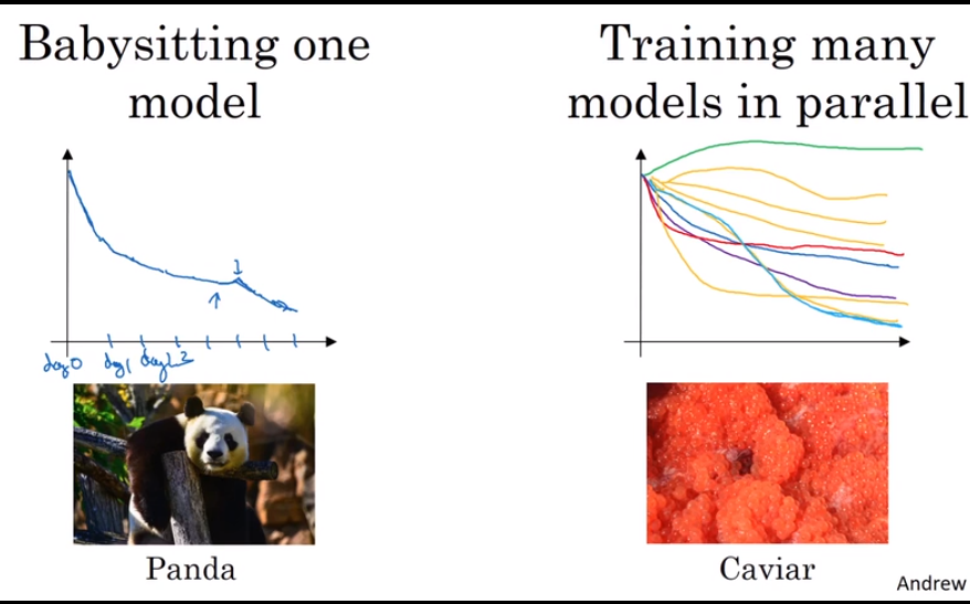
27. Hyperparameters tuning in practice: Pandas vs. Caviar

The two different way of hyperparameters tuning.

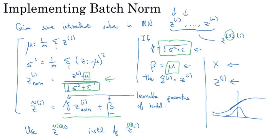
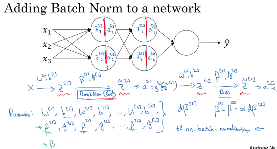
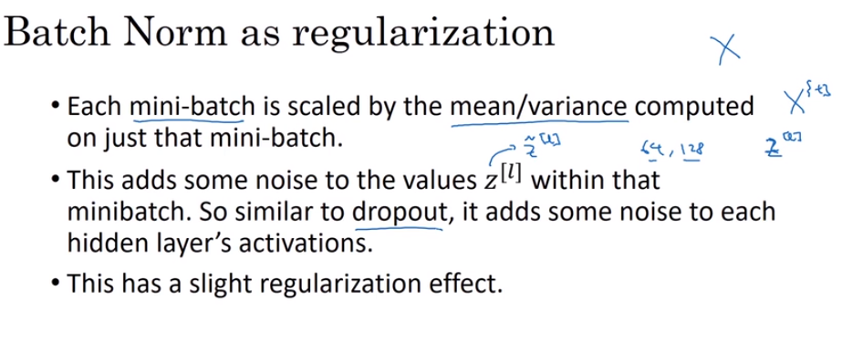
28. Normalizing activations in a network.

30. Why Batch Norm work?

the function of Batch Norm is to control the mean (to zero) and variance (to one) of the input of each hidden layers by transfer the shape of input to normal distribution.

so why we have to control the mean and variance?

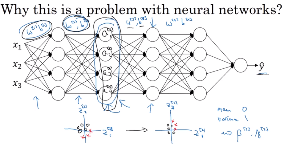
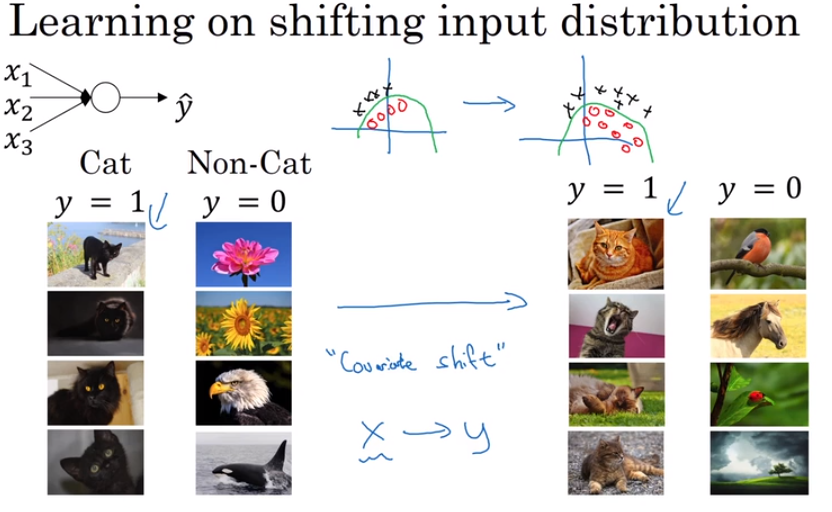
this controlling is to undermine covariate shift which means the precede hidden layers’ parameters updated could put a great influence into the output, affect the latter hidden layers’ parameters, which means in chinese “牵一发而动全身”. It makes the updating of neural networks is unstable and chaos, which I mean when our newest data have a great difference from prior data, the neural network might perform worse.

but using inputs with the shape of normal distribution could avert it.

So the truly meaning of using batch norm is to make each hidden layer more independent.

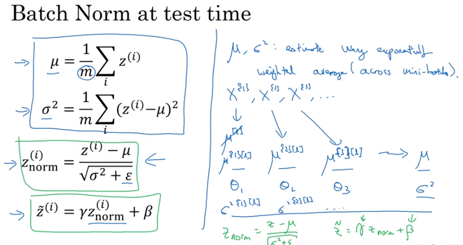
31. Batch norm at test time

In test time, we need other way to calculate mu and sigma

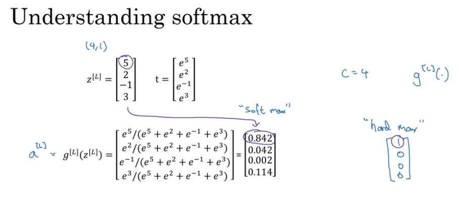
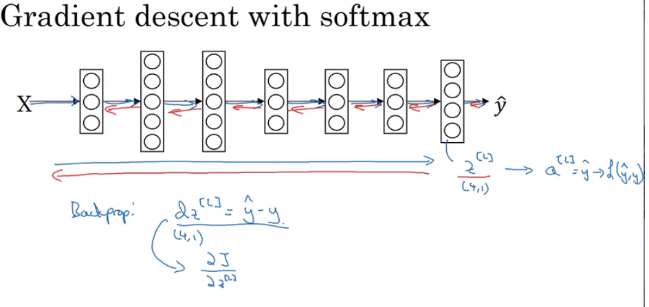
32. Softmax regression

one of generalizations of logical regression

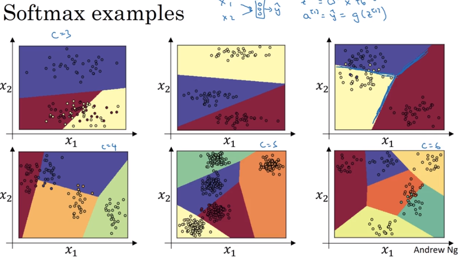
Not just binary classification, but could give a variety of result.

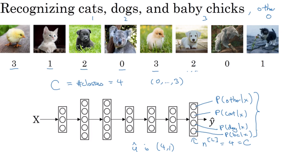
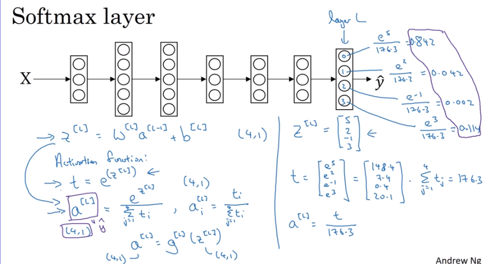
The different is input a vector, output a vector

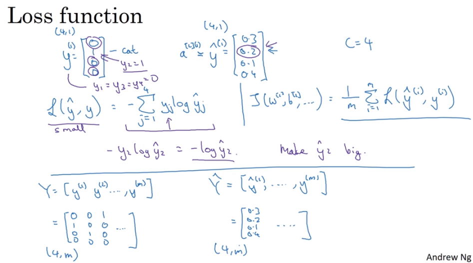
33. Training a softmax classification.

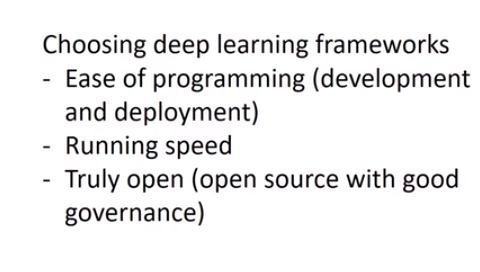
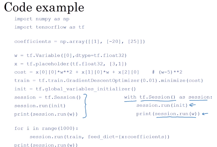
34. Deep Learning frameworks

35. TensorFlow

• Basically using

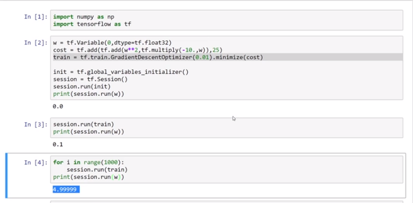
• input data

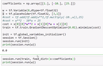
• whole code example

第三课：视频课1-12

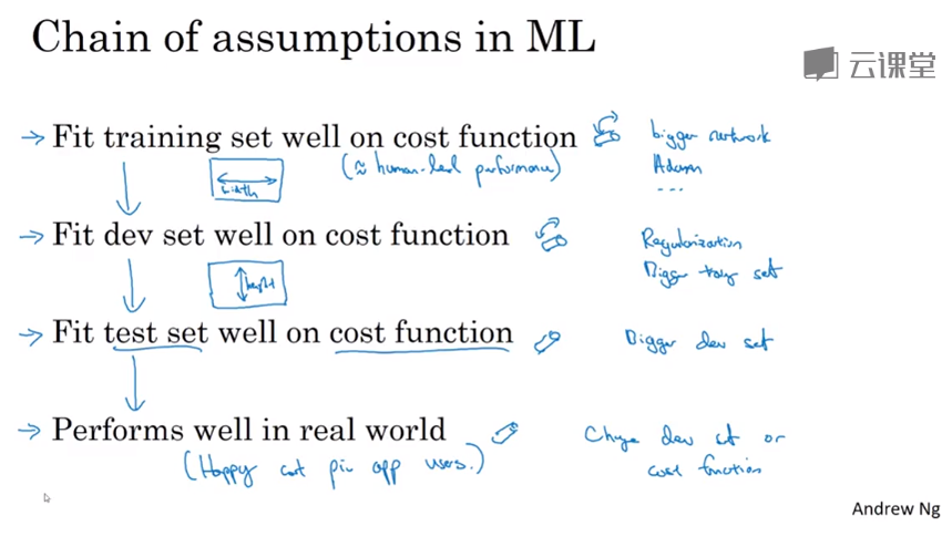
1. Why is ML strategy

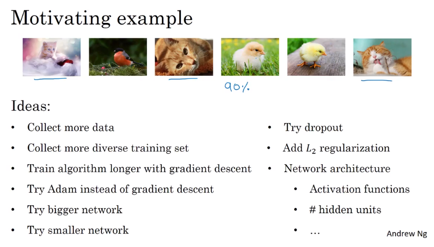
How to choose the best method for improve the performance of ML.

2. Orthogonalization 正交化

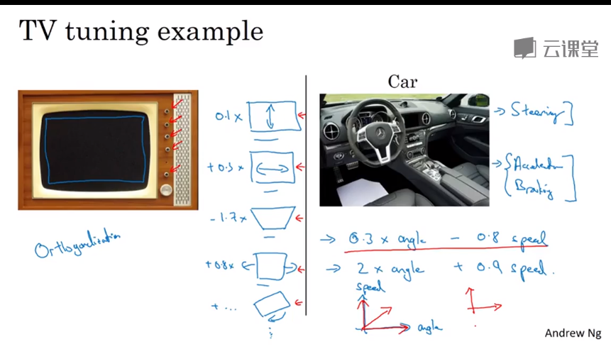
Orthogonalization means let each parameter when it changes will not affect other parameters.

3. Single number evaluation metric 单一数字评估指标

Precision 查准率 of the example that your classifier recognizes as cats, what percentage actually are cats?

Recall 查全率 of all the images that really are cats, what percentage were correctly recognized by your classifier?

F1 Score the mixture of P and R

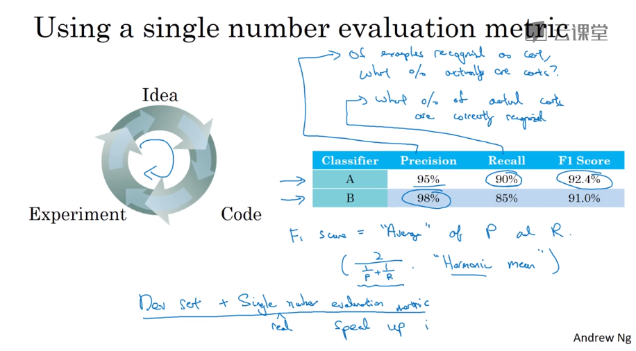
By using the average, it make us easy to figure out which classifier is performing better than others classifier overall.

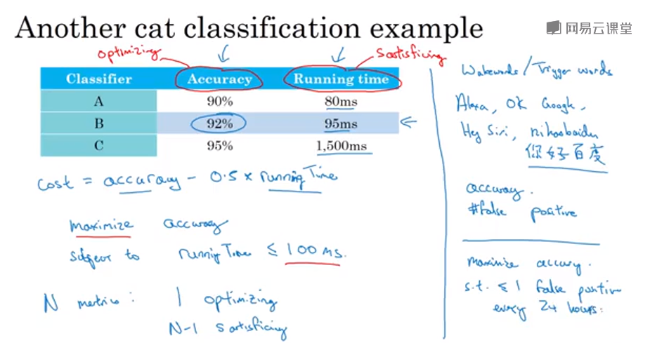
4. Satisficing and optimizing metrics.

We should care about both accuracy and running time.

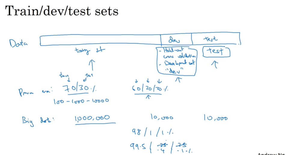
5. Train/dev/test distributions

One bad idea: using not really randomly choosed sets for equally distributing.

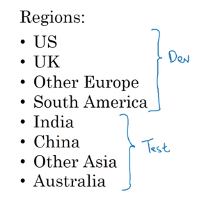
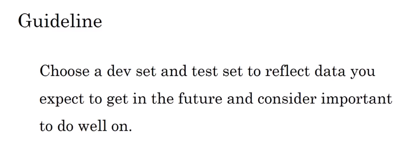
==A real great idea is to set the dev and test sets both have data containing all apperent conditions such as region in this example.==

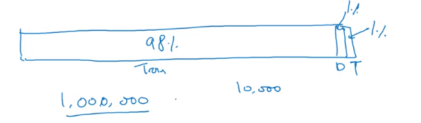
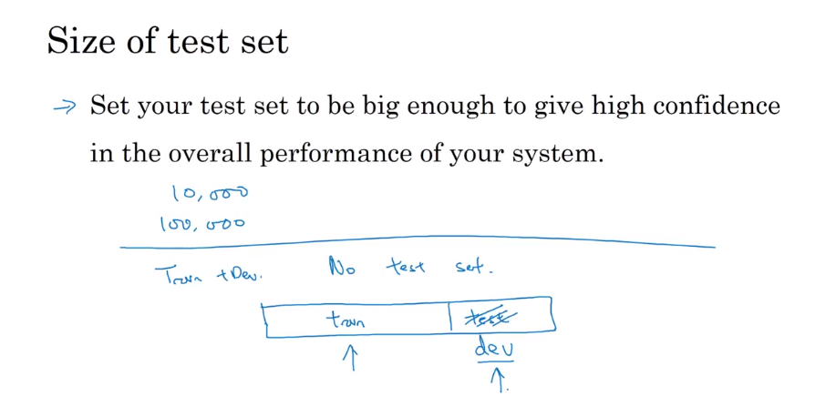
6. Size of dev and test sets

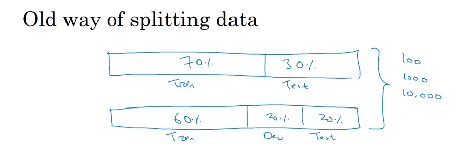
But in the era of big data, we have to change ways to decide the size of dev and test sets

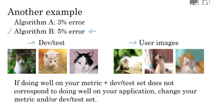
7. When to change dev/test sets and metrics

Sometimes, one algorithm maybe perform greater than others, but it will output some unacceptible results when it goes wrong. So we may not use it because of terrible consequence because of the algorithm’s low-possible but inexorable blunder.

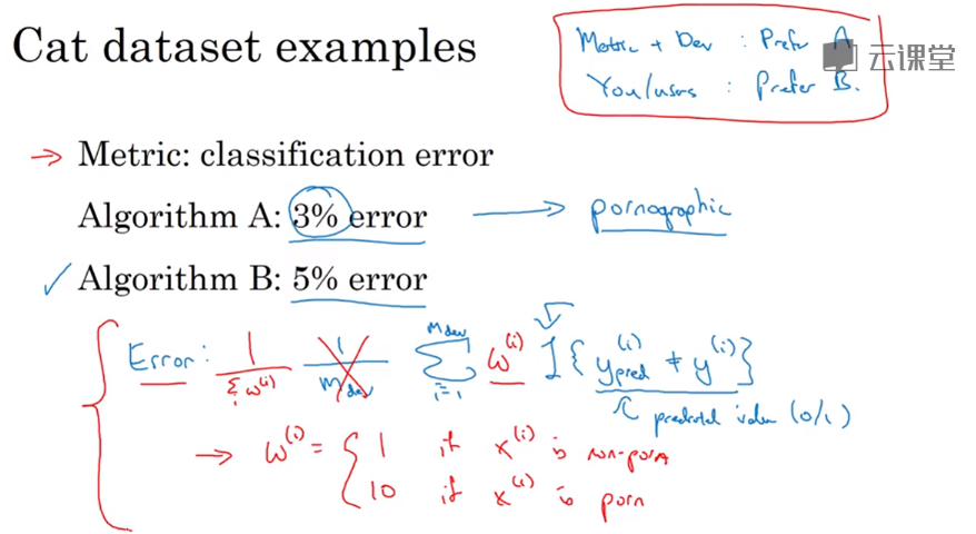
Here are our usage which weighting the index of each error emerging to make us get the best algorithm which fits our individually special demand

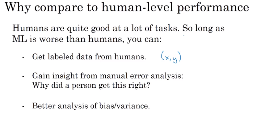
8. Why human-level perormance

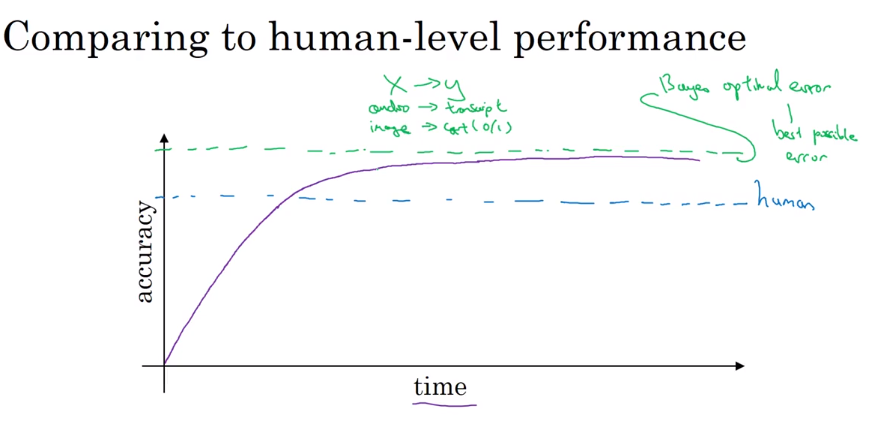
Bayes optimal error, or Bayesian optimal error, or Bayes error for short is the very best theoretical function for mapping from x to y.

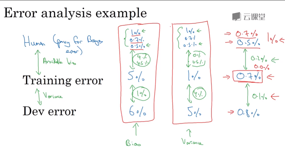
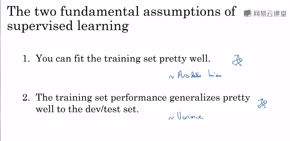
9. Avoidable bias

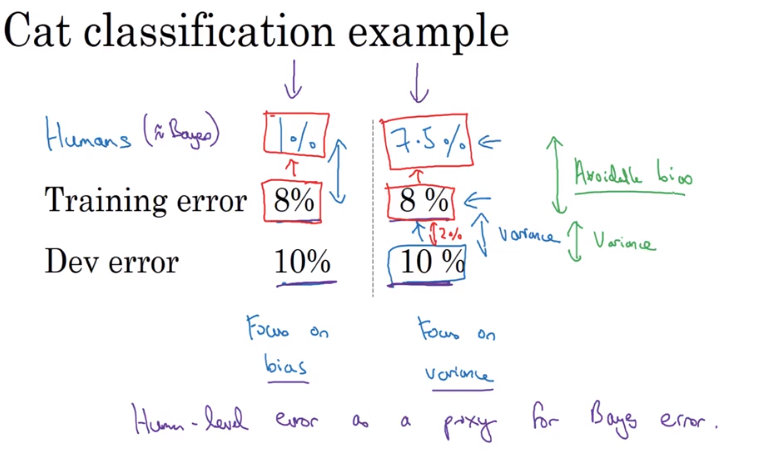
10. Understanding human-level performance

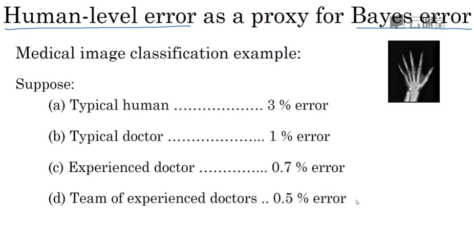
How should you define human-level error?

**Of course we should use the best performance as human-level error, to substitute or estimate the Bayes error, but it this case, when our AI do not perform good enough, choose using anyone to be Bayes error is meaningless. **

When avoidable bias is non-ignorable, we should keep eyes on Bias, otherwise we should pay attention to Variance.

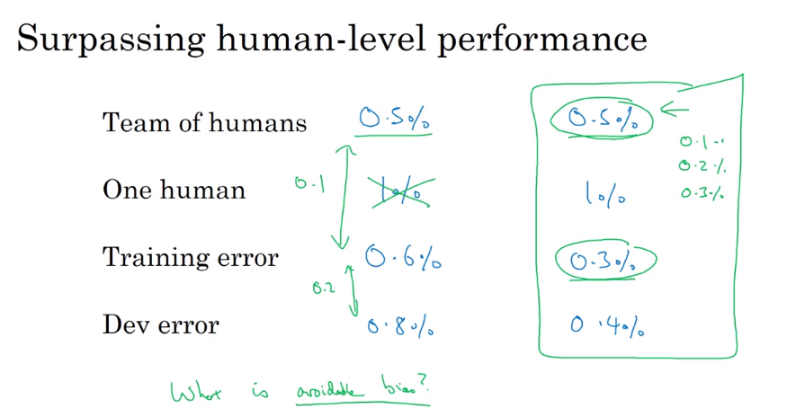
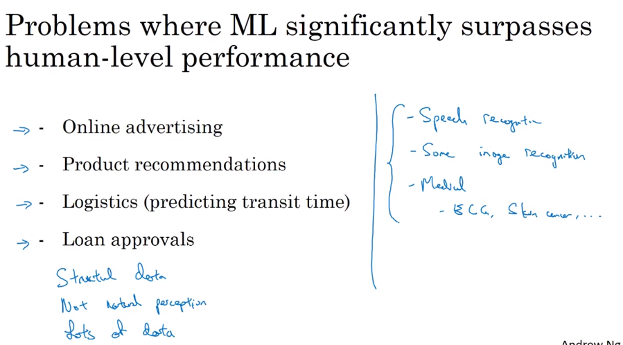
11. Surpassing human-level performance

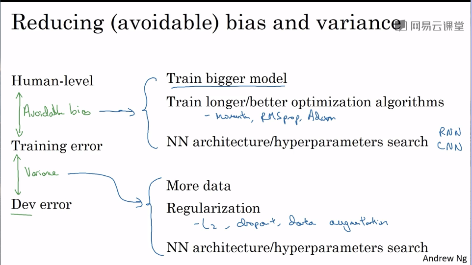
12. Improving your model performance

第三课：视频课13-22

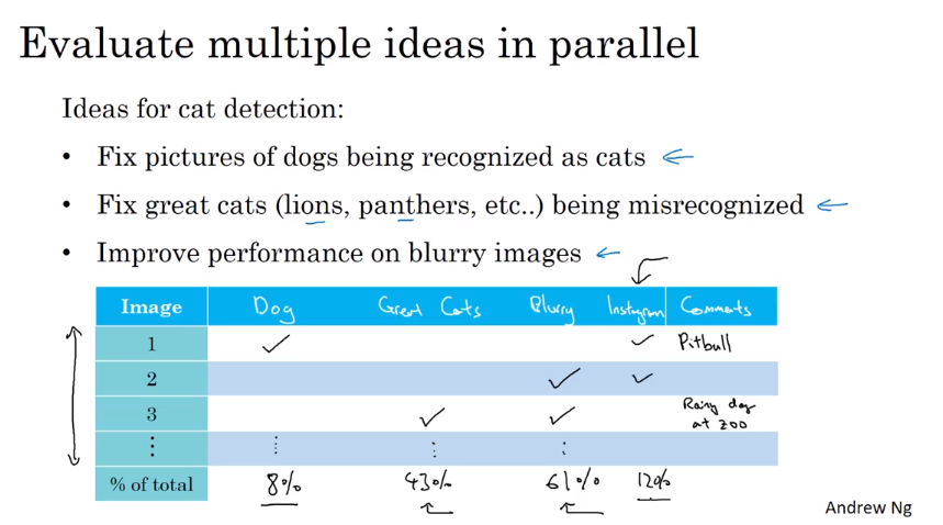
13. Carring out error analysis 错误分析

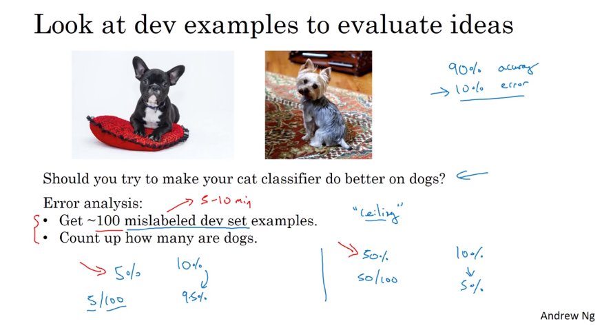
1. Found how the error may be caused.
2. Figure out the possible reasons.
3. Use a sheet to statistic.

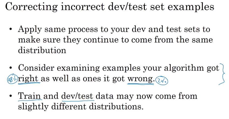
14. cleaning up incorrectly labeled data

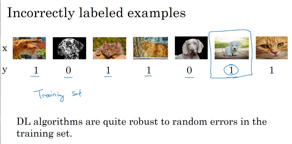
So long as the total data set is big enough, the random error is ok, but the systematic errors is not ok.

15. Build your first system quickly, then iterate

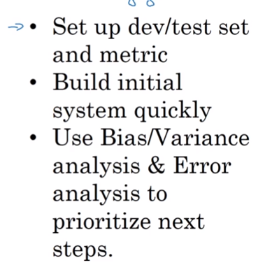
Guideline: Build a system first, and iterate.

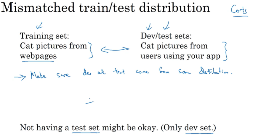
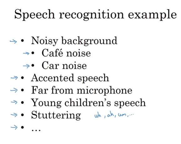
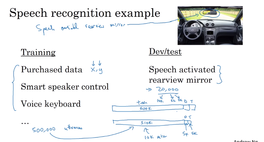
16. Training and testing on different distributions.

There are two ways to solve it.

1. Merge them and shuffle.

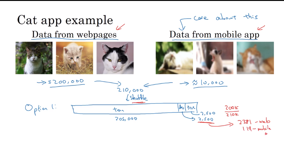
2. use basis dataset to train, and the real worthy data to test.

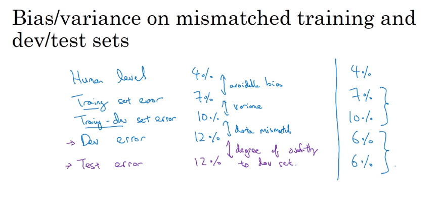
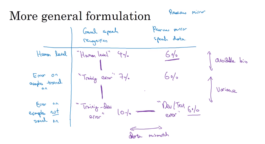
17. Bias and Variance with mismatched data distributions

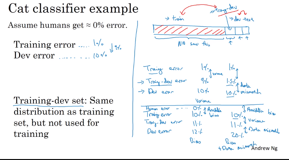
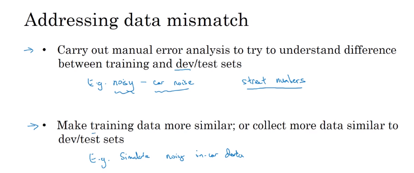
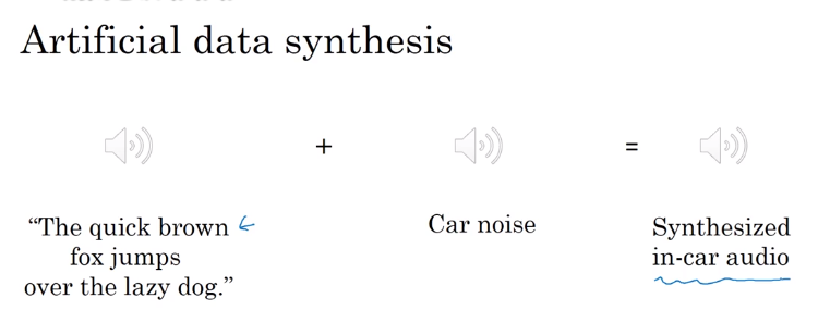
18. Addressing data mismatch

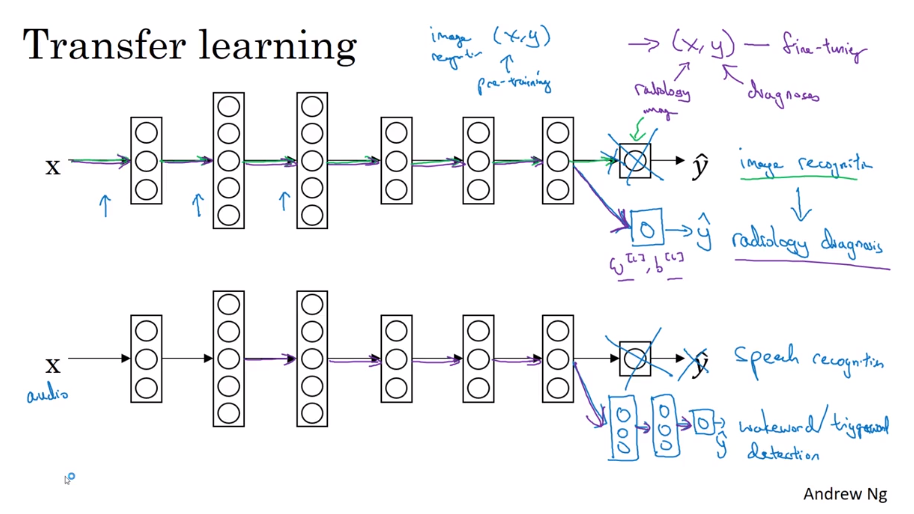
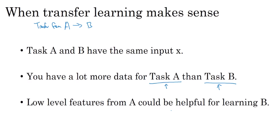
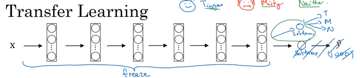
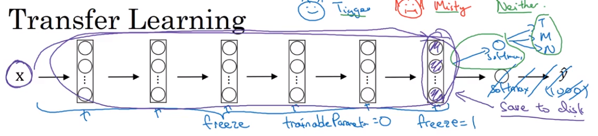
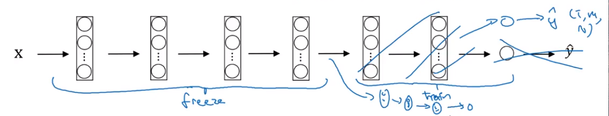
19. Transfer learning 迁移学习

Use old knowledge in new task

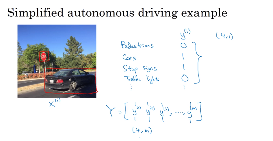
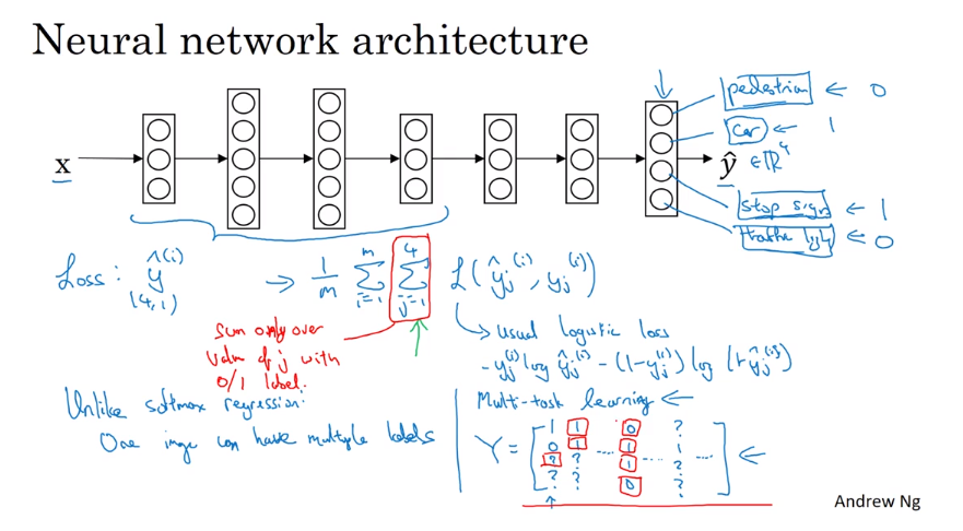
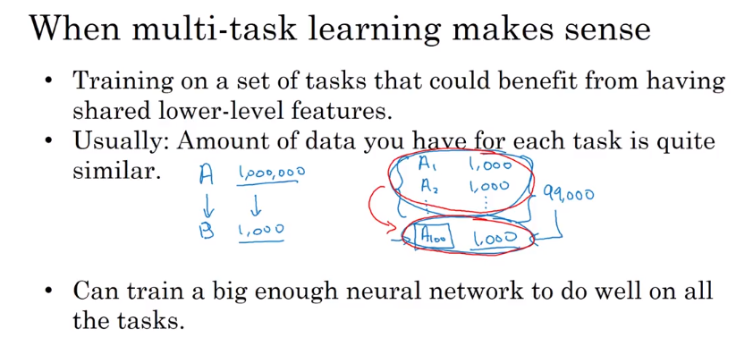
20. Multi-task learning 多任务学习

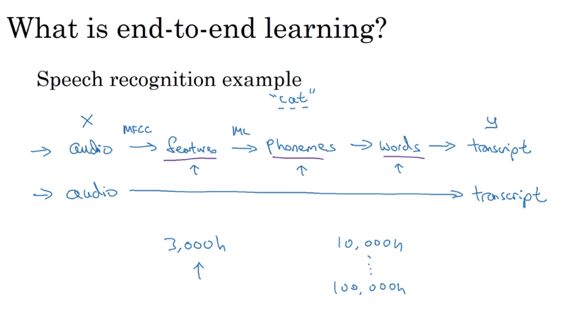
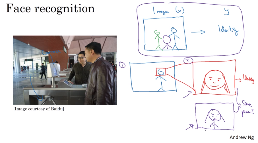
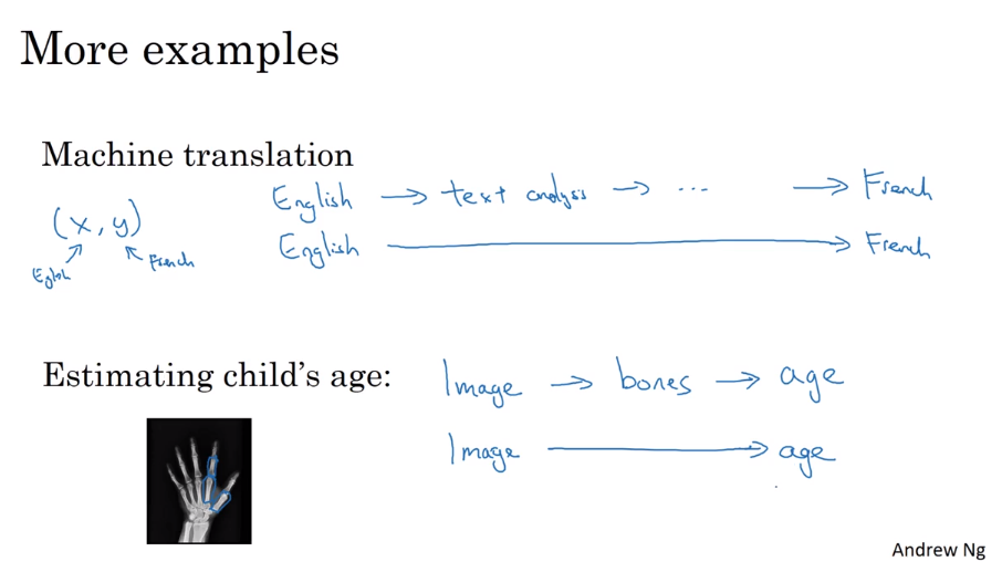
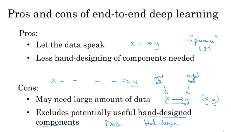
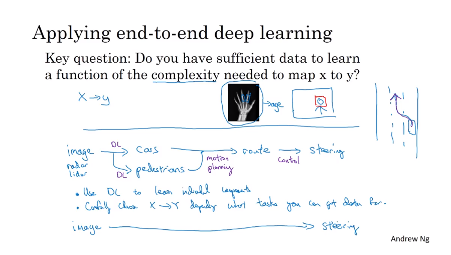
21. End-to-End deep learning 端对端深度学习

22. Whether to use end-to-end deep learning

第四课：视频课1-11

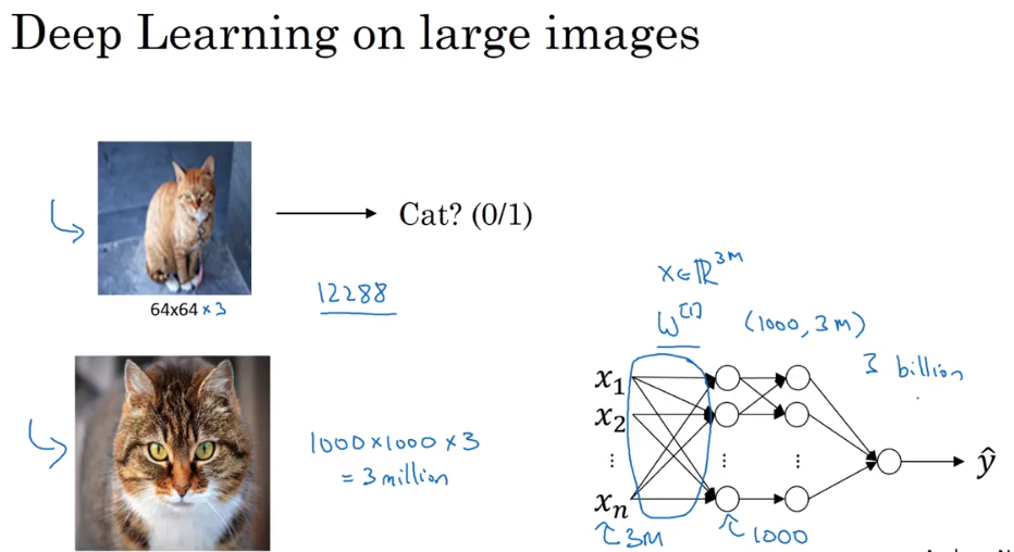
1. Computer Vision

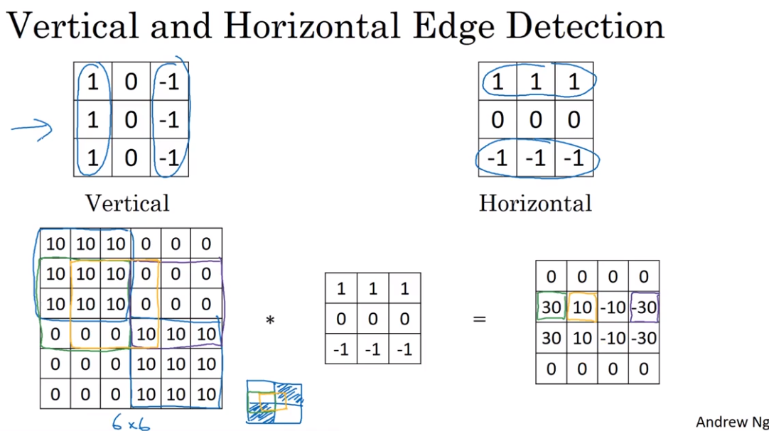
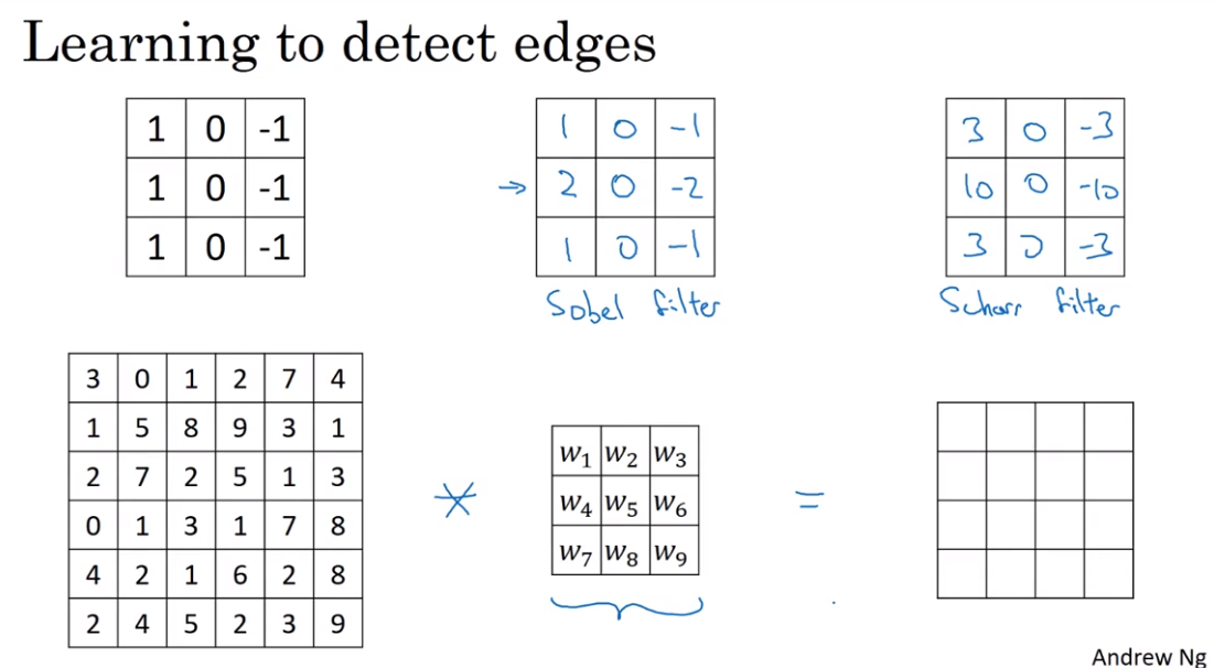
2. Edge Detection

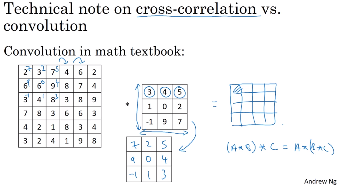
Convolution 卷积

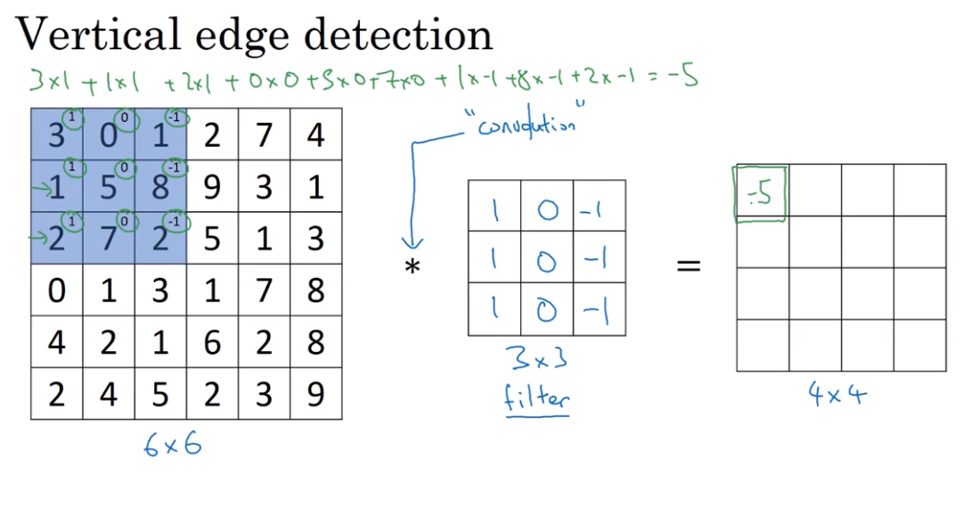
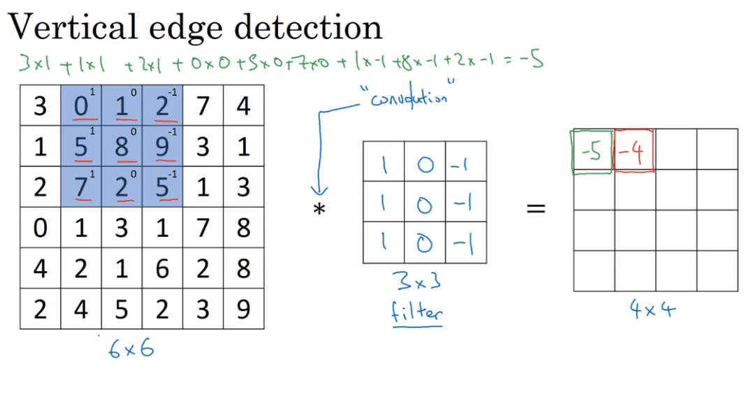
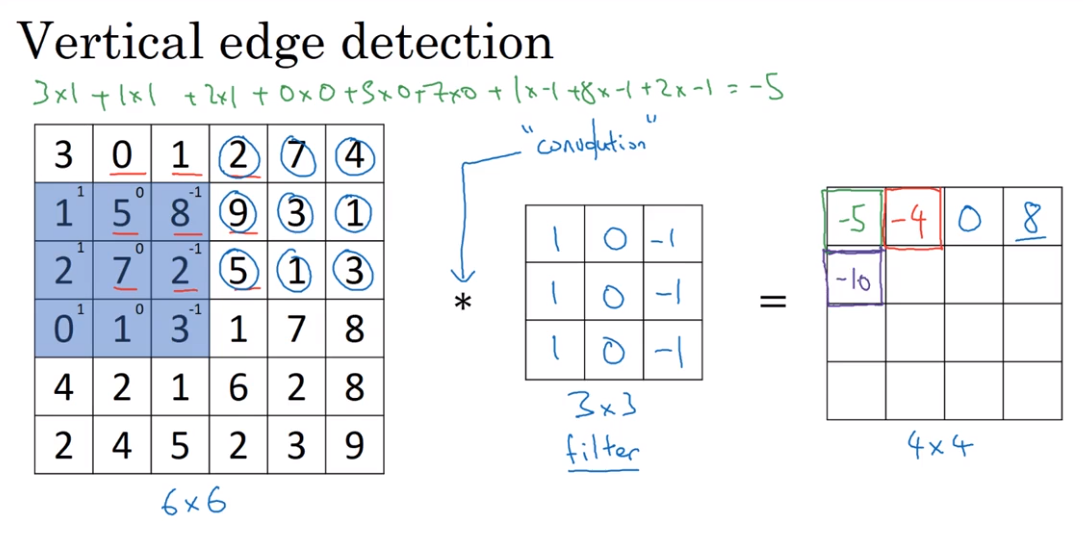
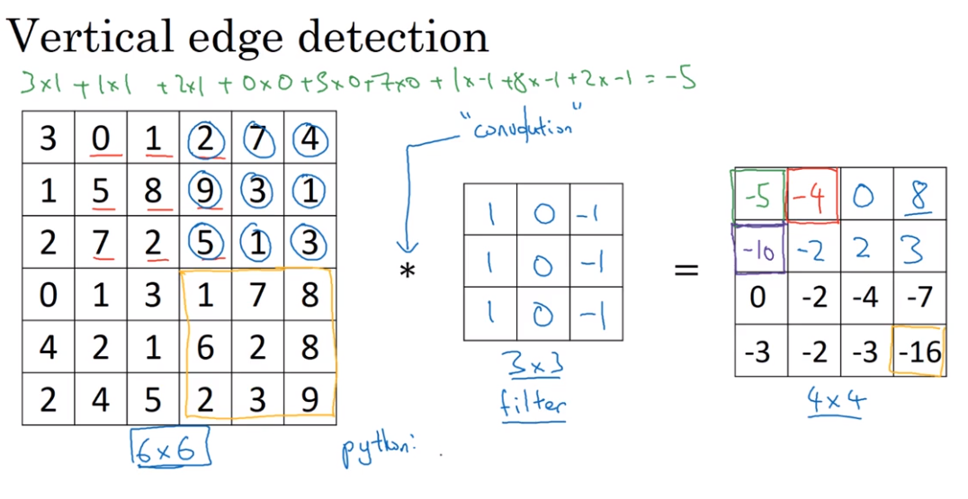
The usage of convolution in Vertical edge detection

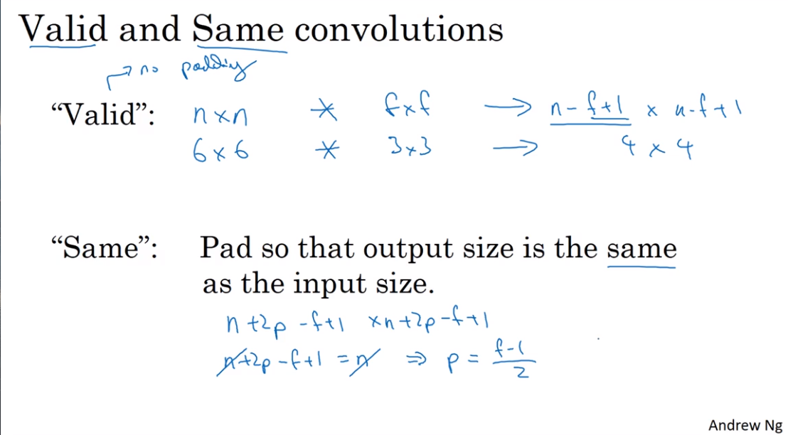
4. Padding

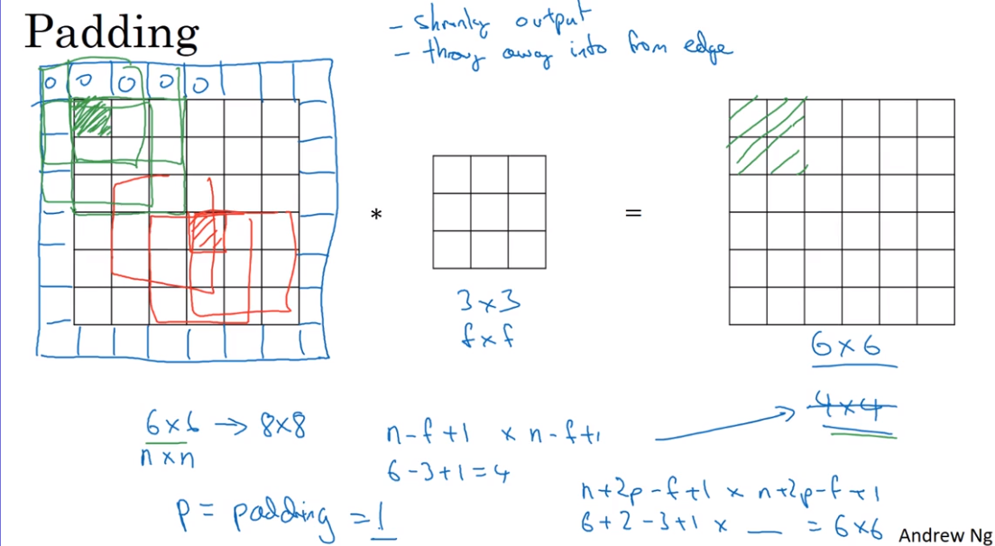
Two strategy of Padding convolutions

We usually use odd-numbered f for building filter

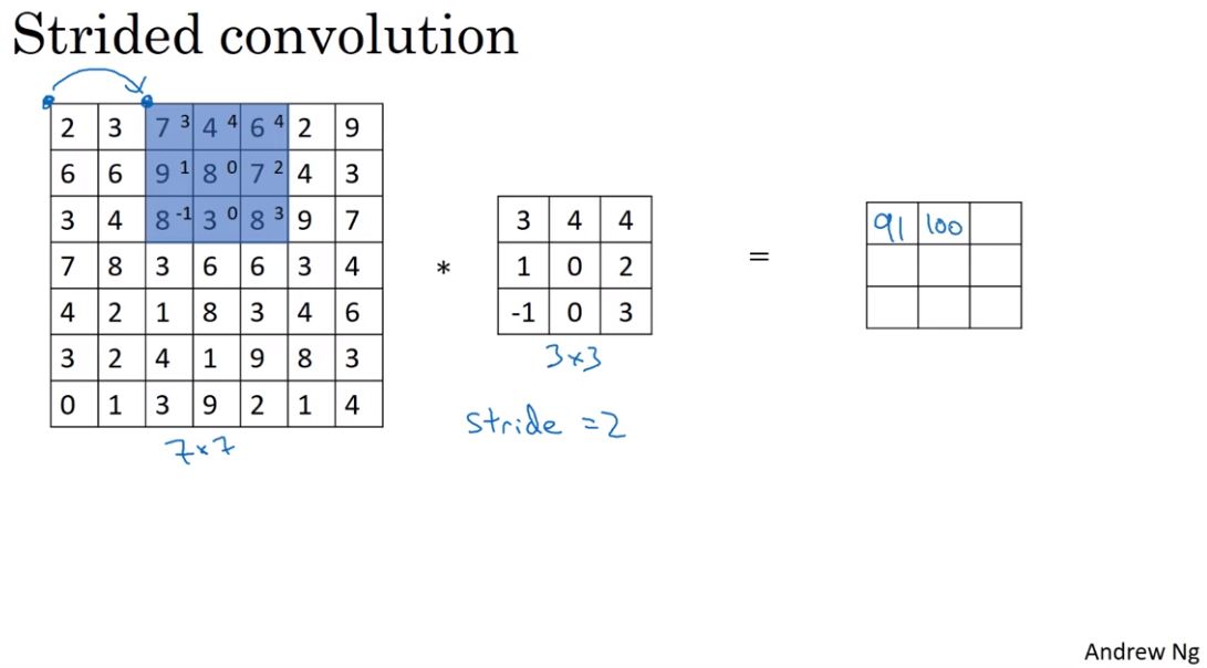
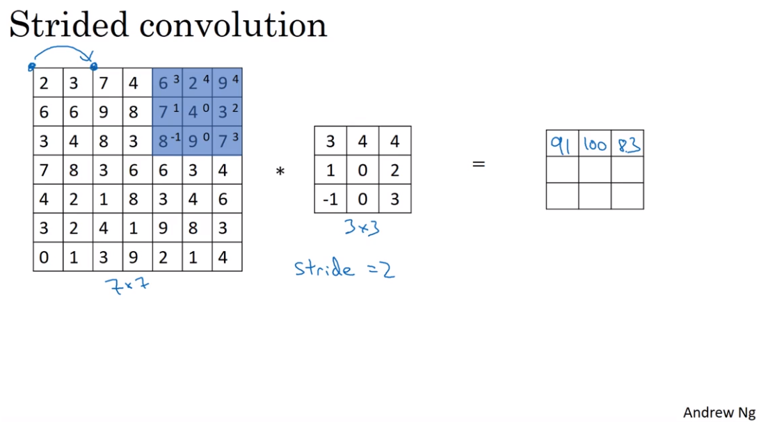
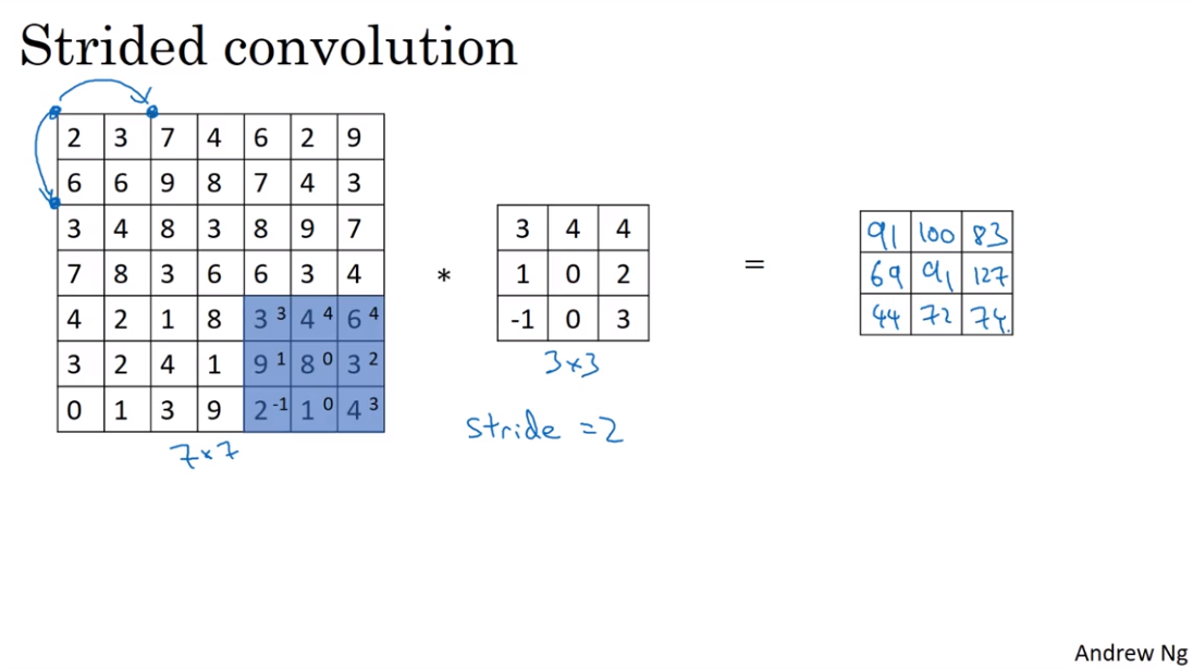
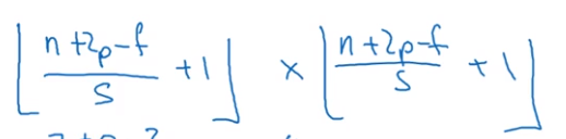
5. Strided convolution

6. Convolution over volumes

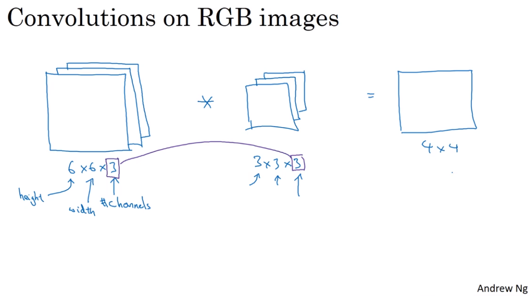
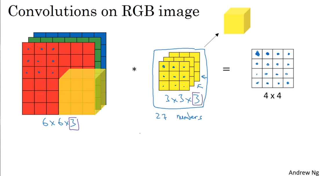
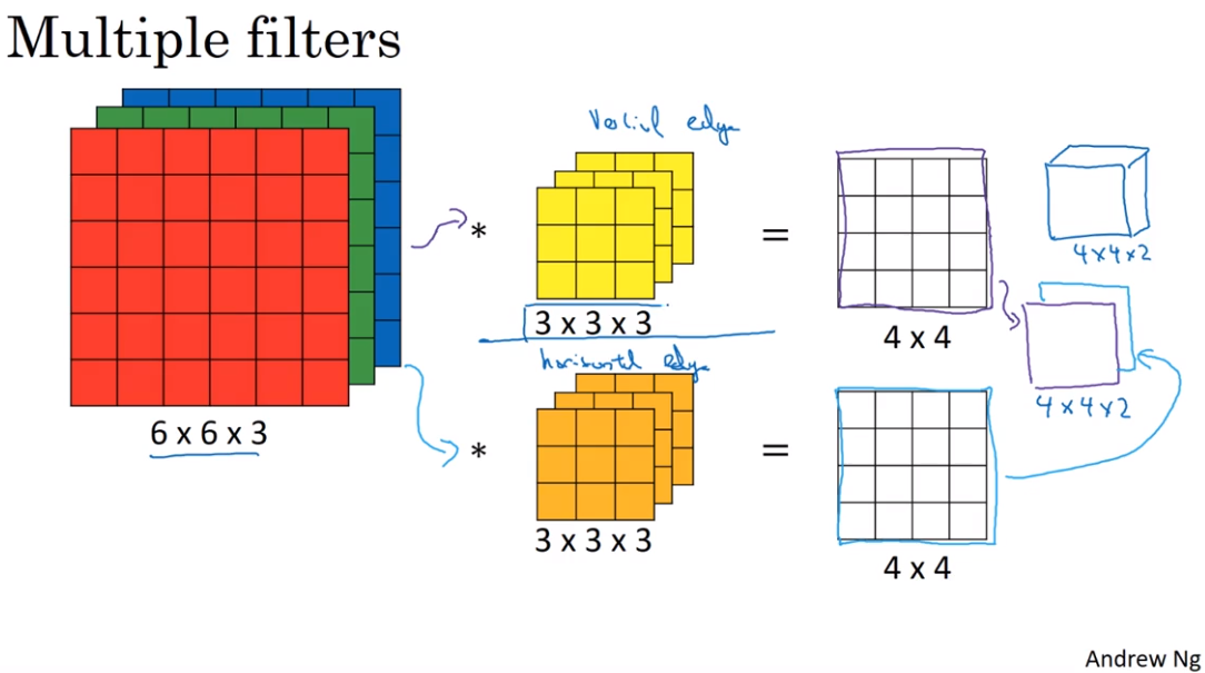
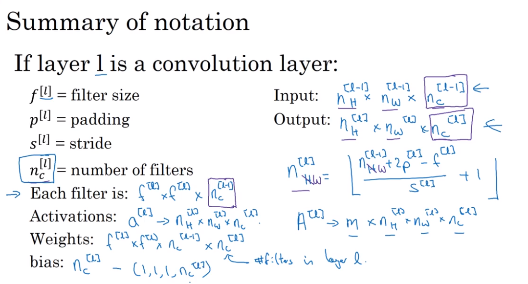
7. One layer of convolutional neural network

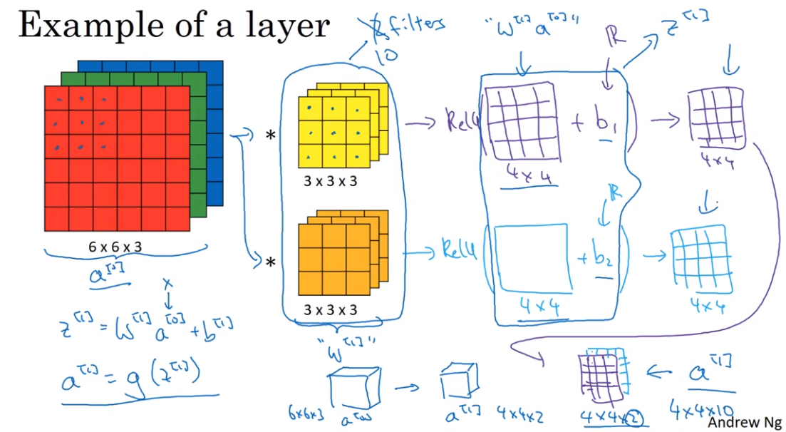
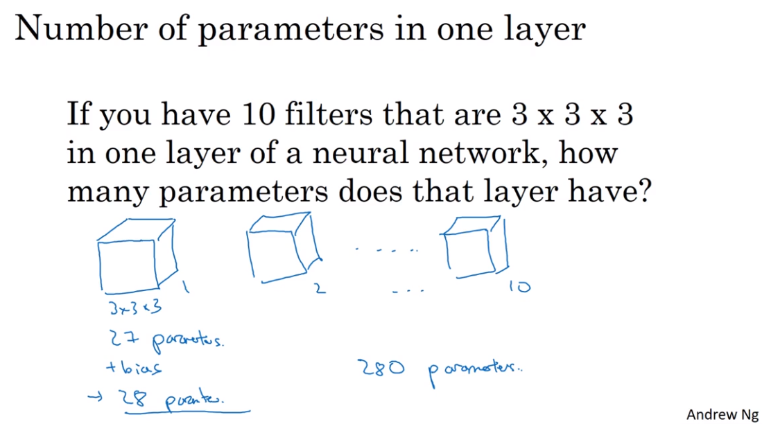
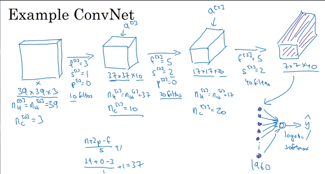
An Example of ConvNet

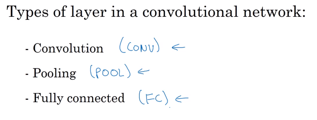
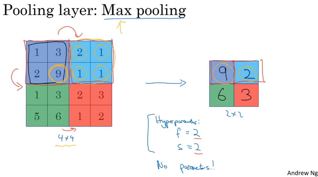
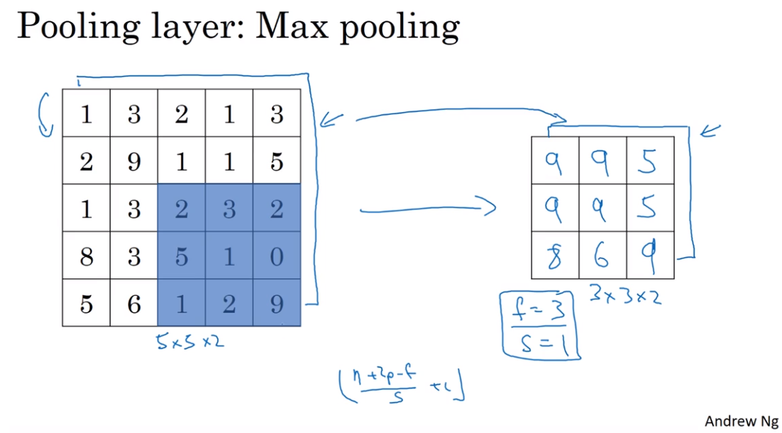
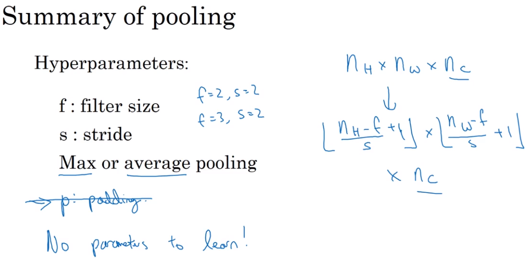
9. Pooling layers 池化层（汇合层）

Use Pooling layers to reduce the size of their representation to speed up computtion, as wel as to some of the features it detects a bit more rebust. 缩减模型大小，提高计算速度，同时提高所提取特征的健壮性

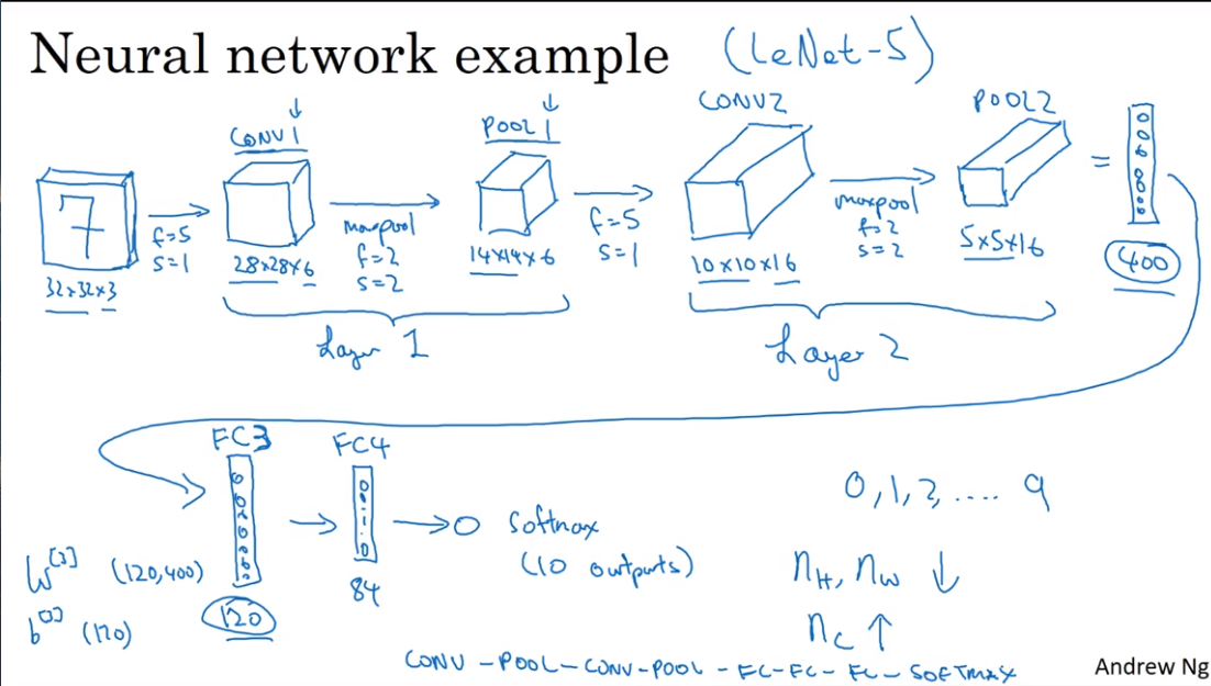
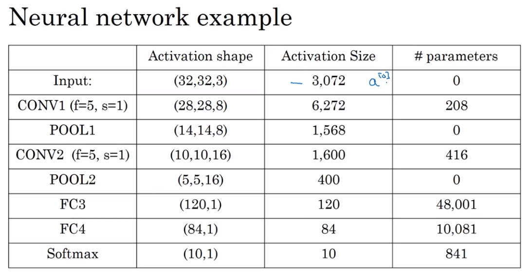
10. Neural network example

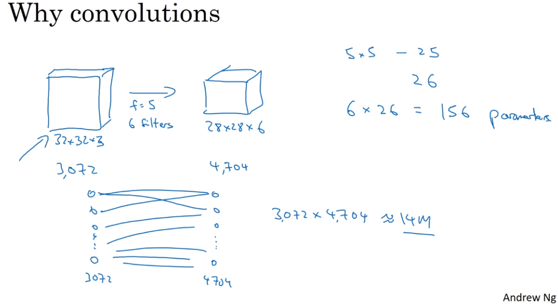
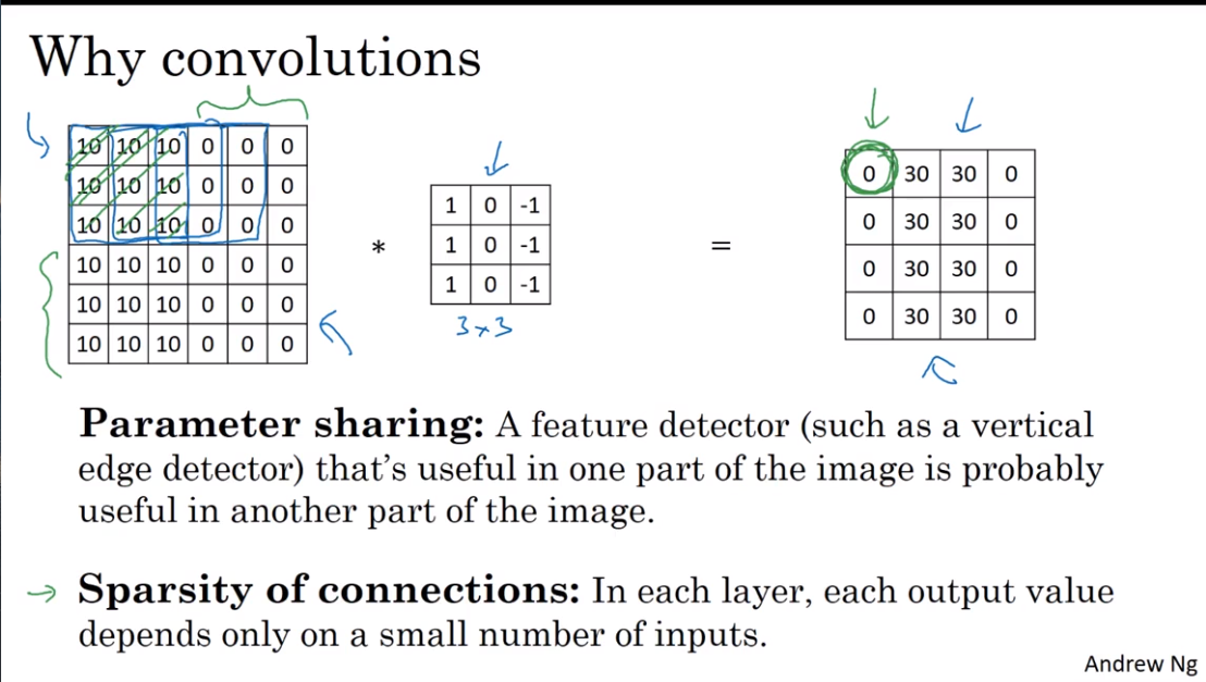
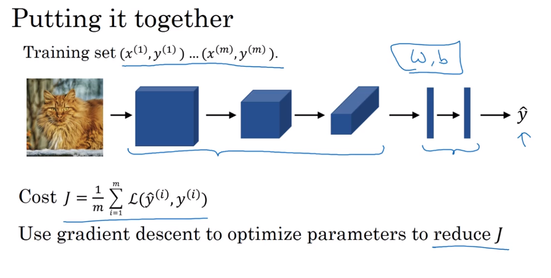
11. Why convolution?

第四课：视频课12-22

12. Why look at cases studies?

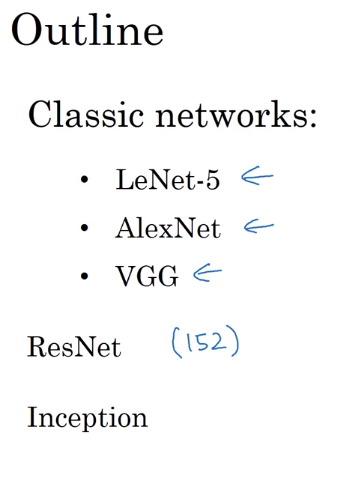
13. Classic networks

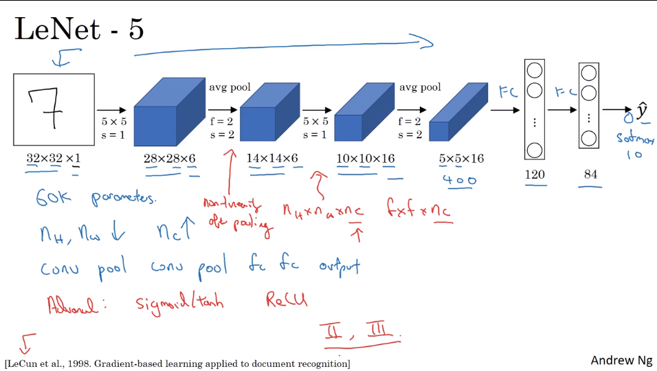
• LeNet - 5 : Recognize the number written by hand

• Alex Net

Input a picture, return a series.

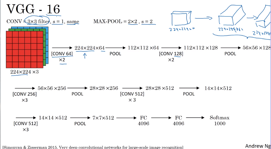
• VGG - 16

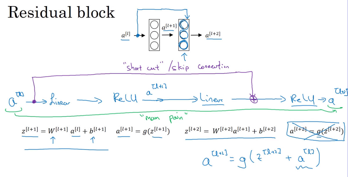
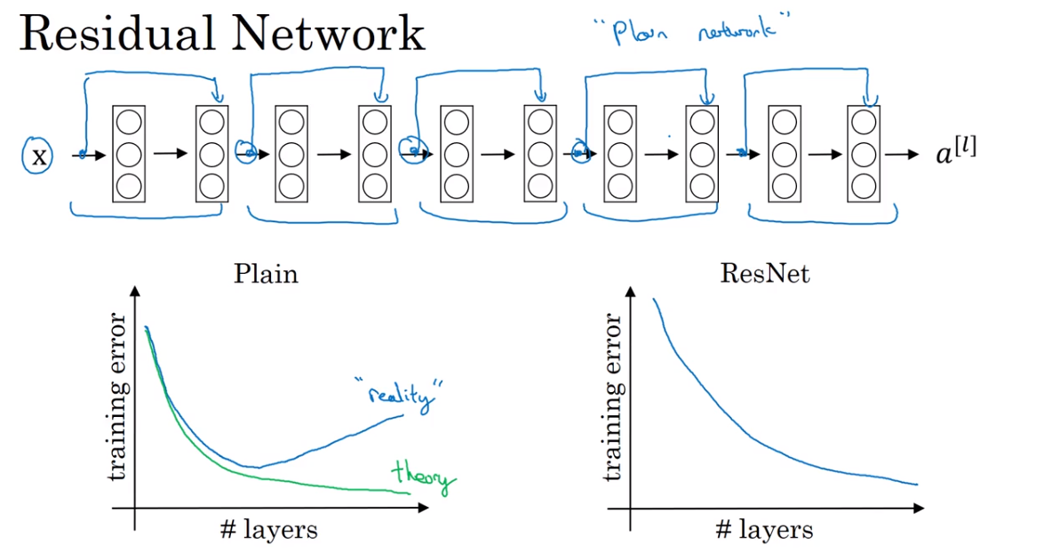
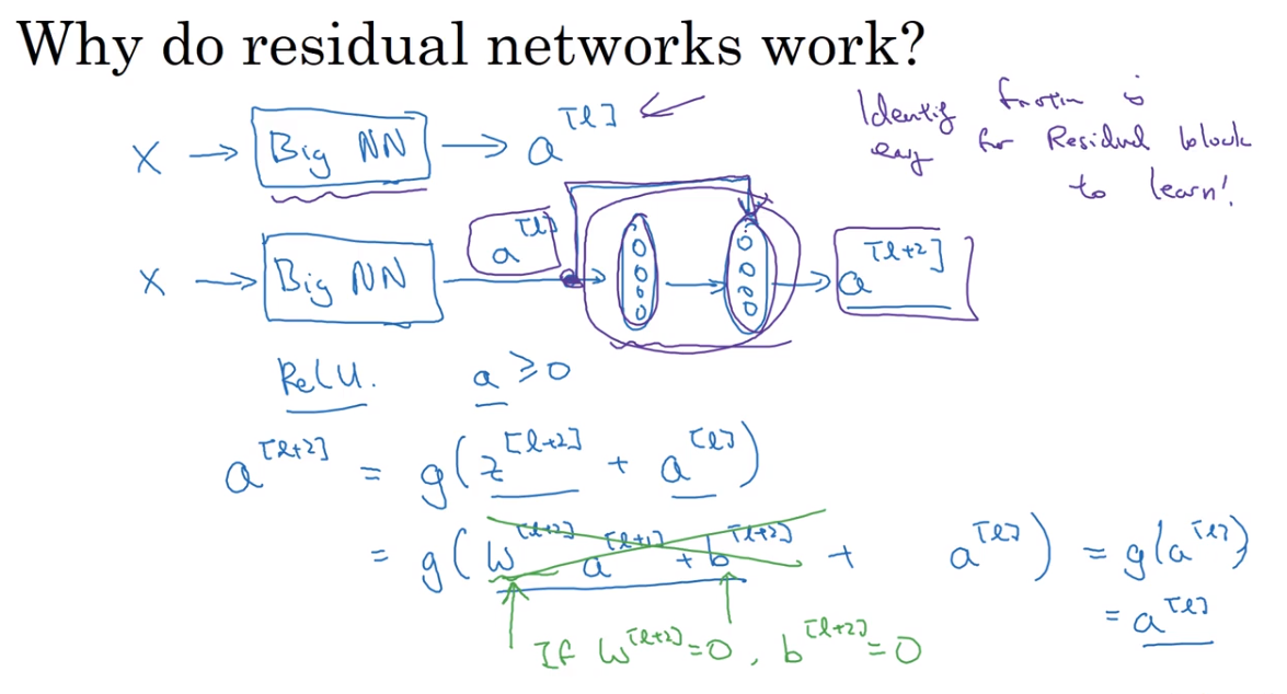
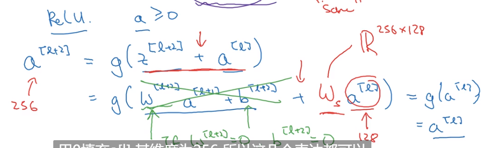
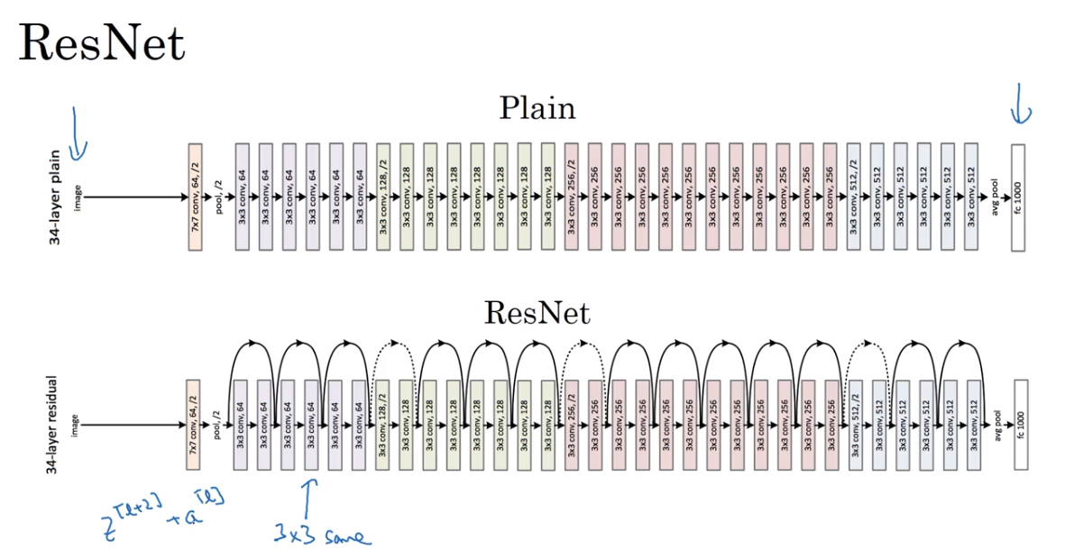
14. Residual Network — Res Net

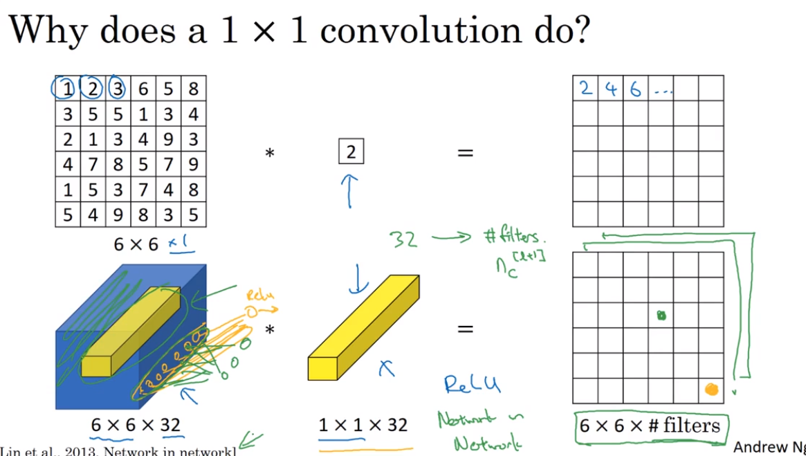
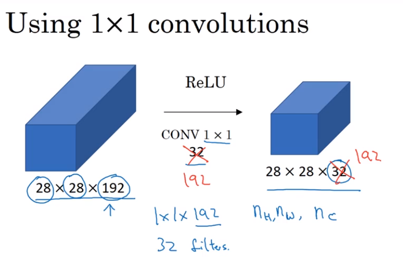
16. Network in Network and 1 * 1 convolutions

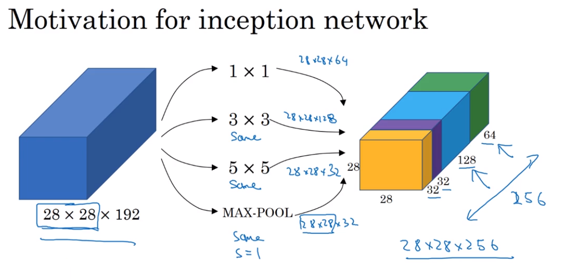
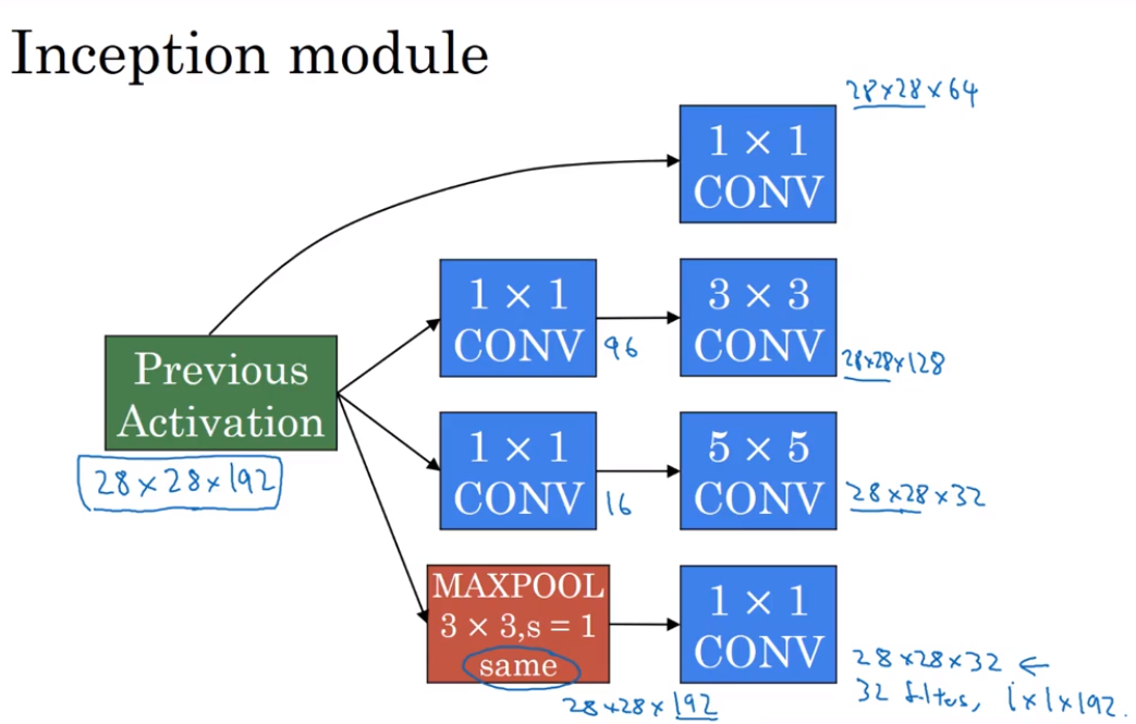
17. Inception Network Motivation

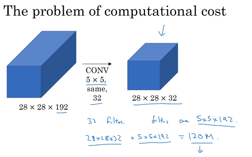
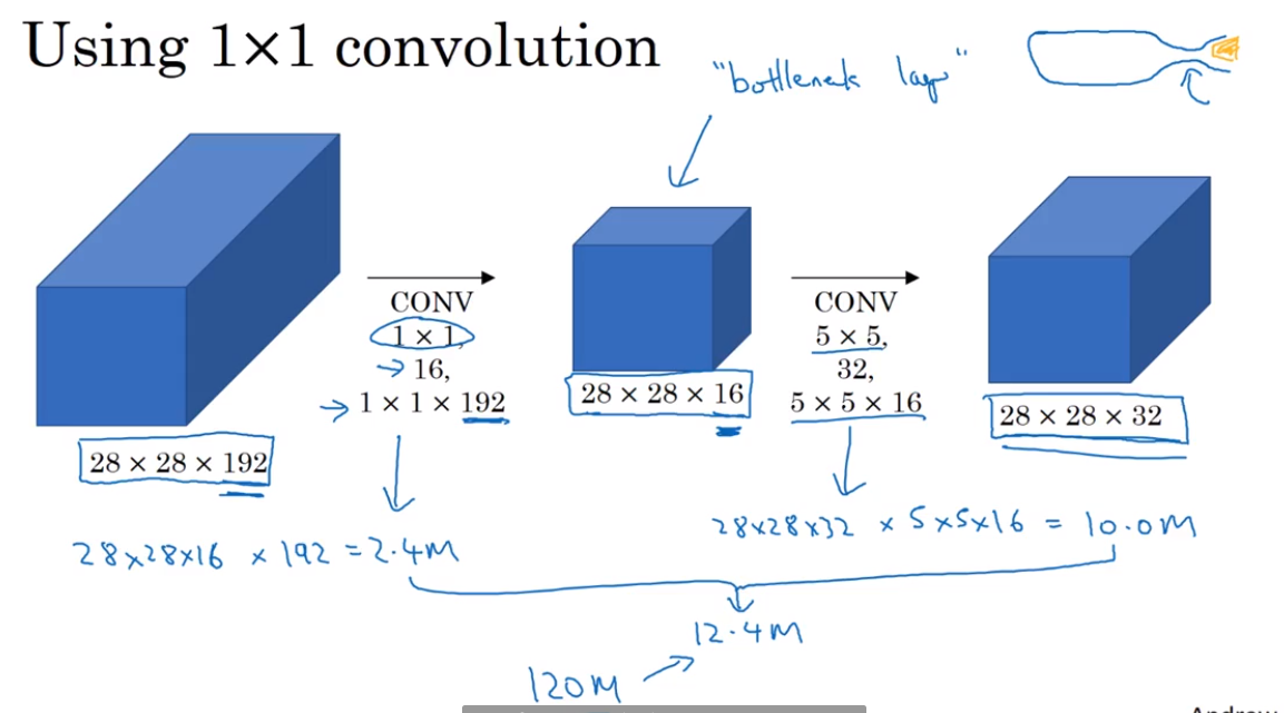
1*1 convolution use to reduce the size of third layers

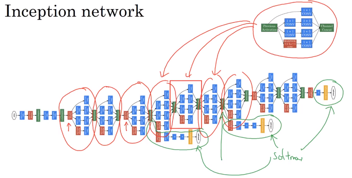
18. Inception Network

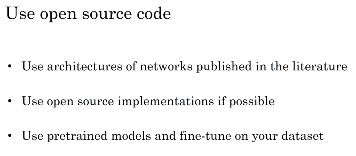
19. Using open-source implementations

Github

20. Transfer Learning

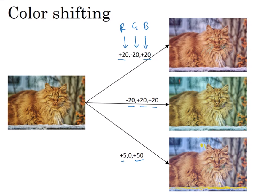
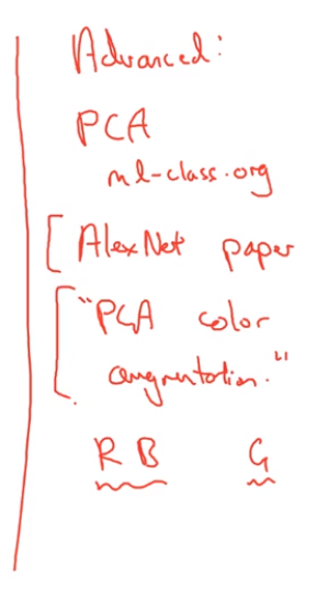
21. Data augmentation

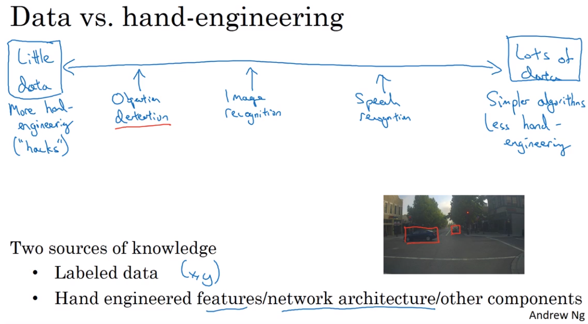
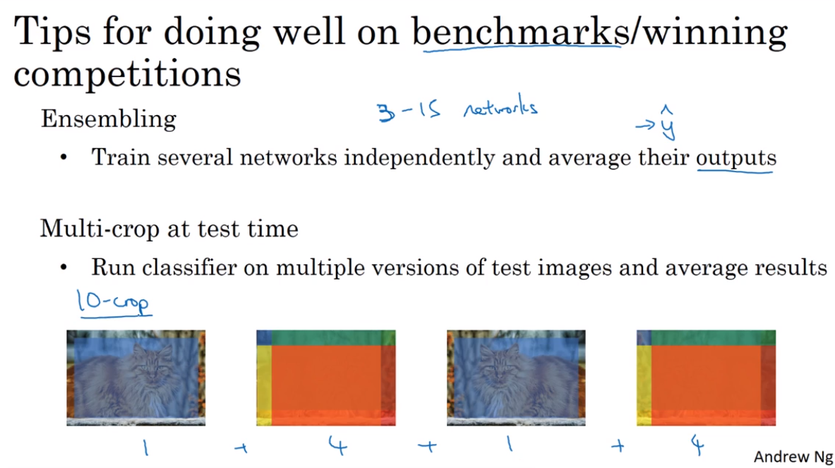
22. The state of computer vision

第四课 视频课22-32

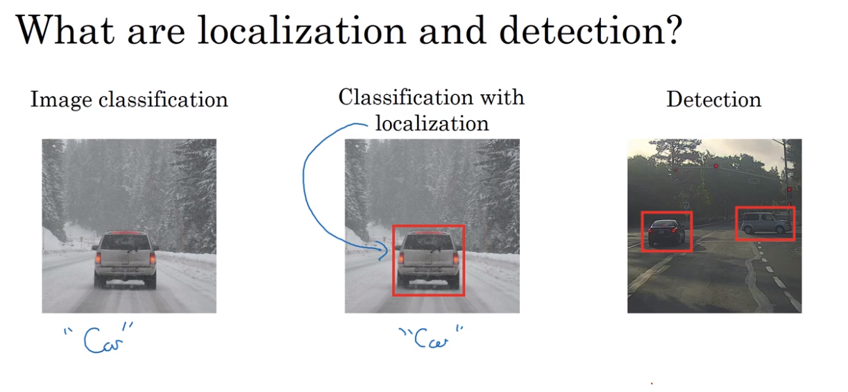
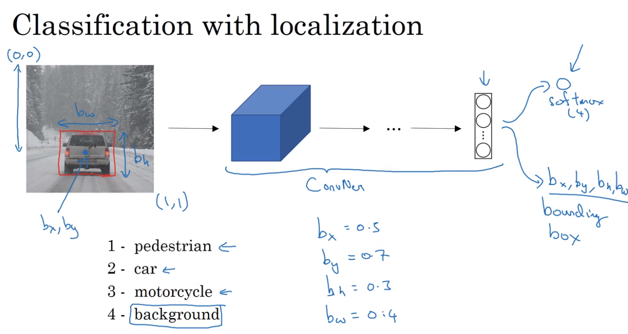
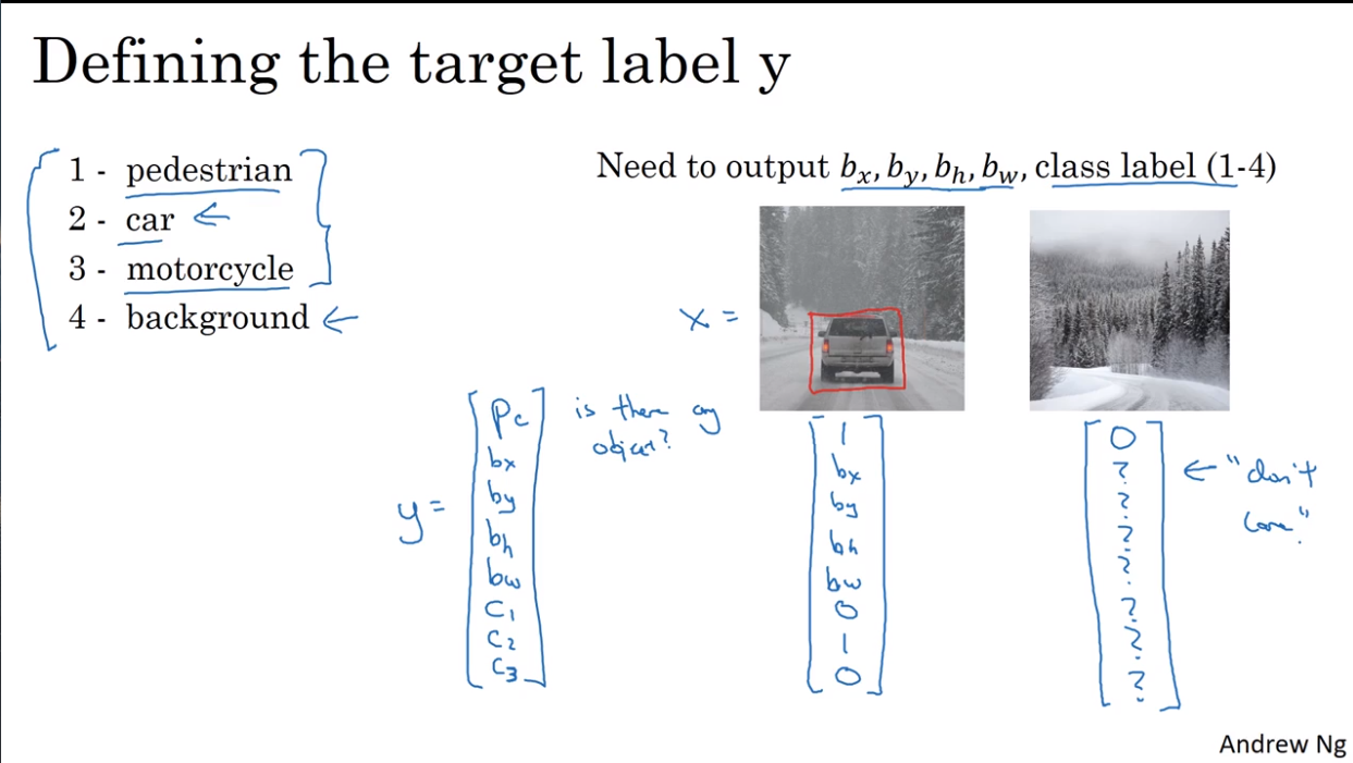
22. Object localization

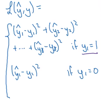
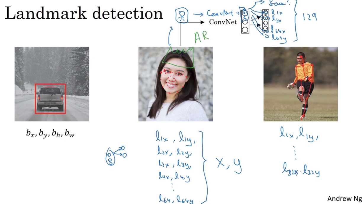
23. Landmark detection

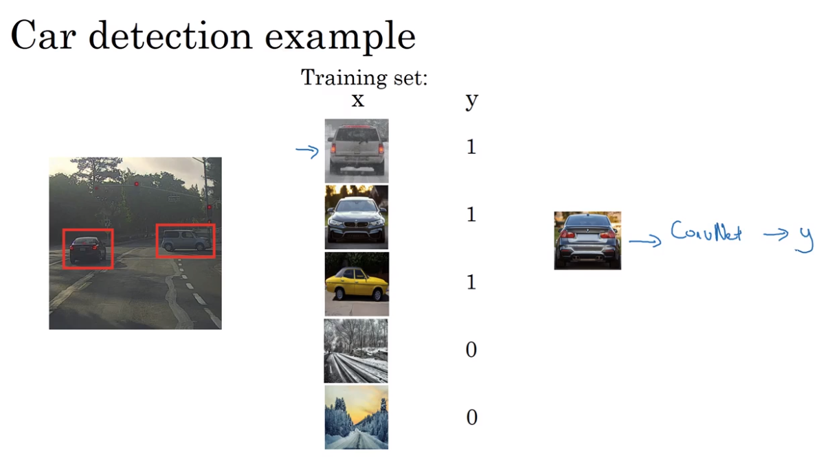
24. Object detection

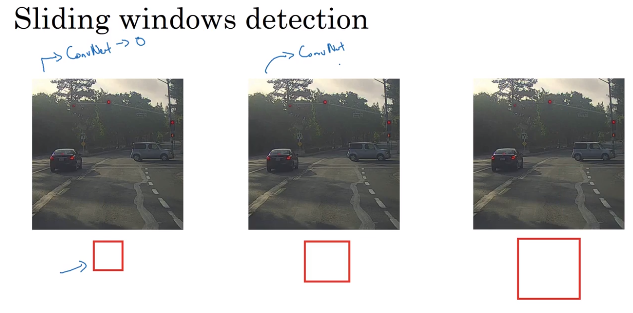
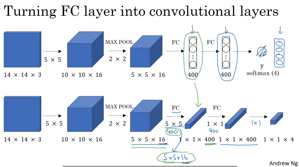
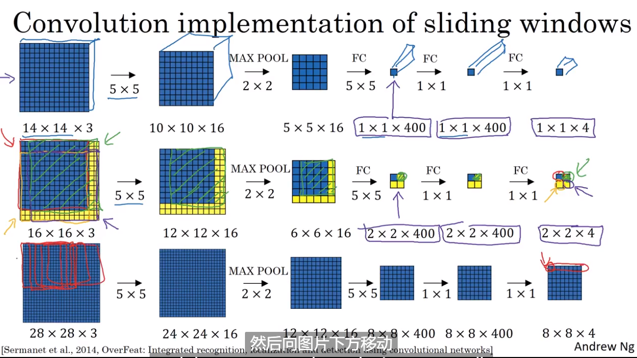
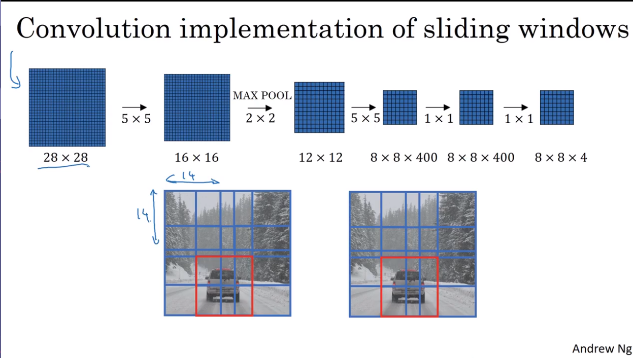
25. Convolutional implementation of sliding windows

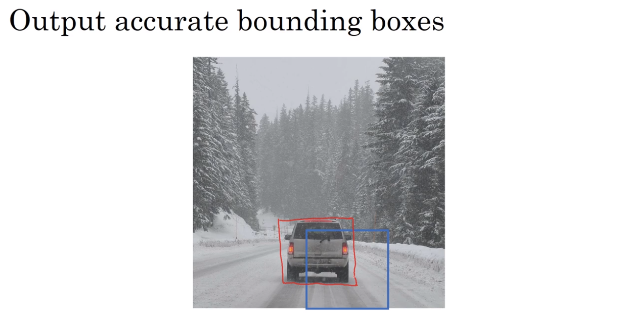
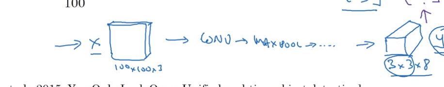
27. Bouding box prediction

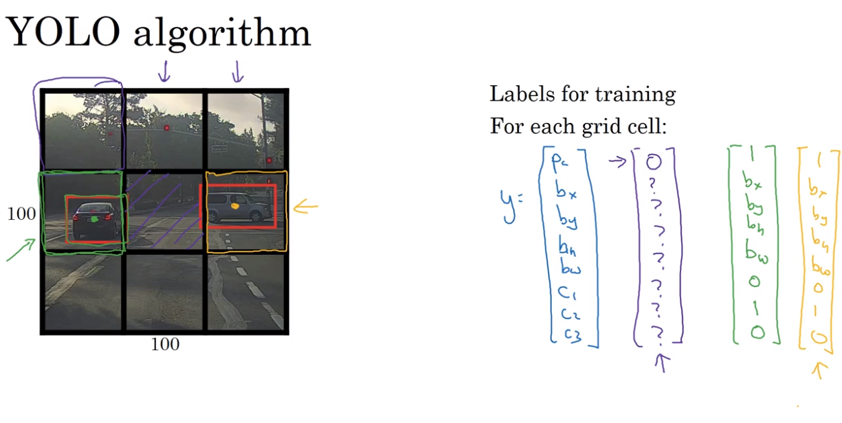
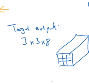
YOLO algorithm

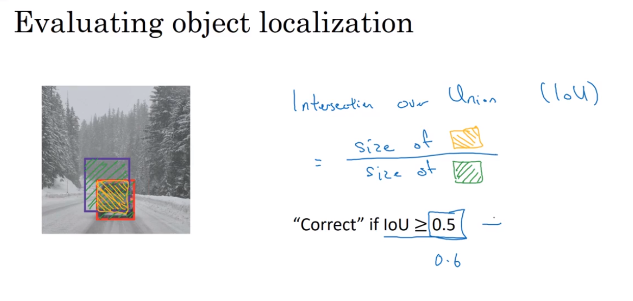
28. Intersection over union 交并比

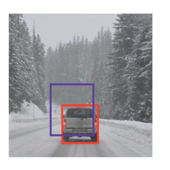
Is it good enough or too bad?

We have to use a algorithm to evaluate it.

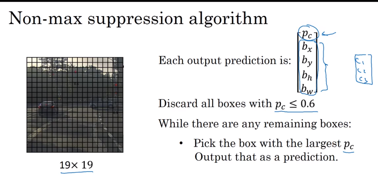
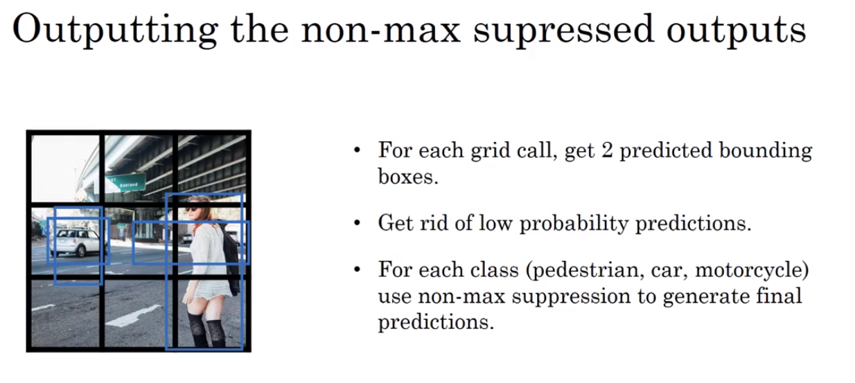
29. Non-max suppresion 非极大值抑制

One result only be detected once.

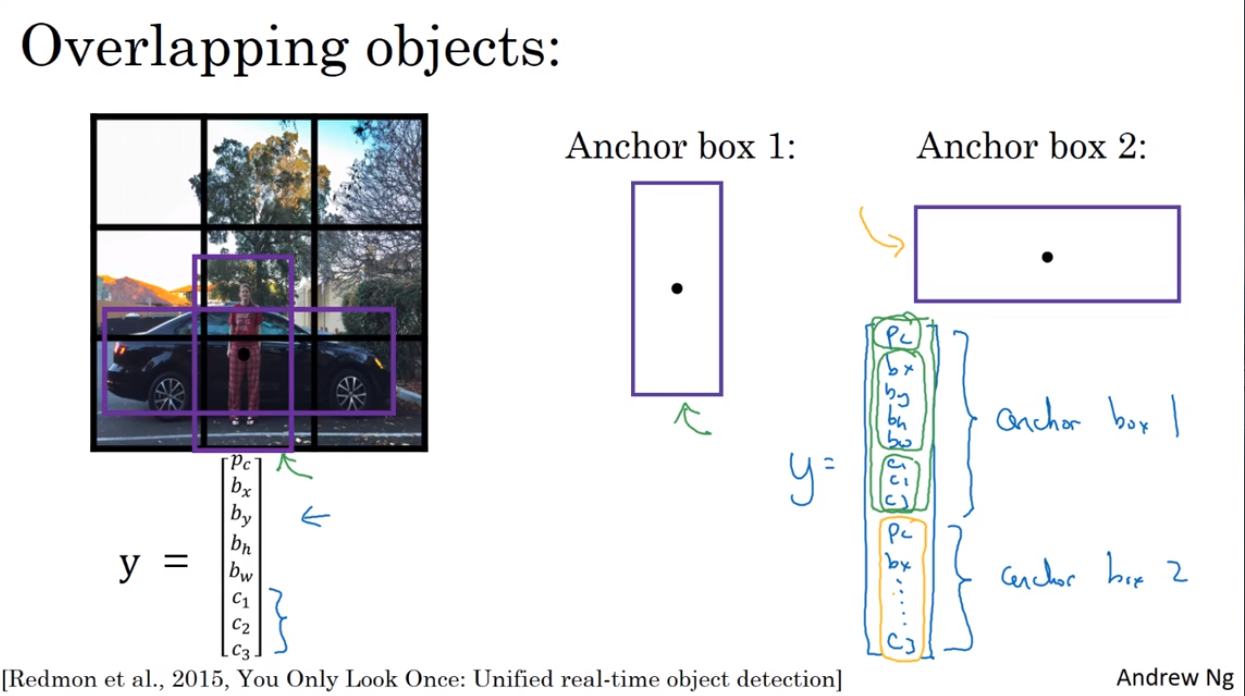
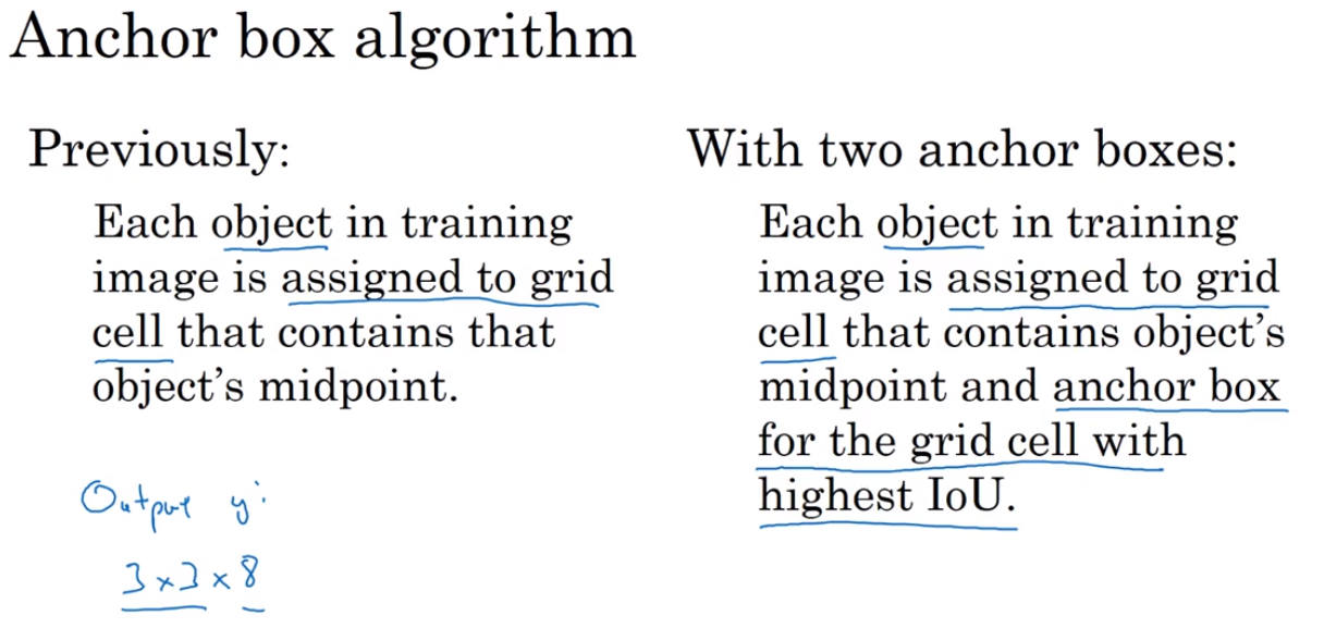
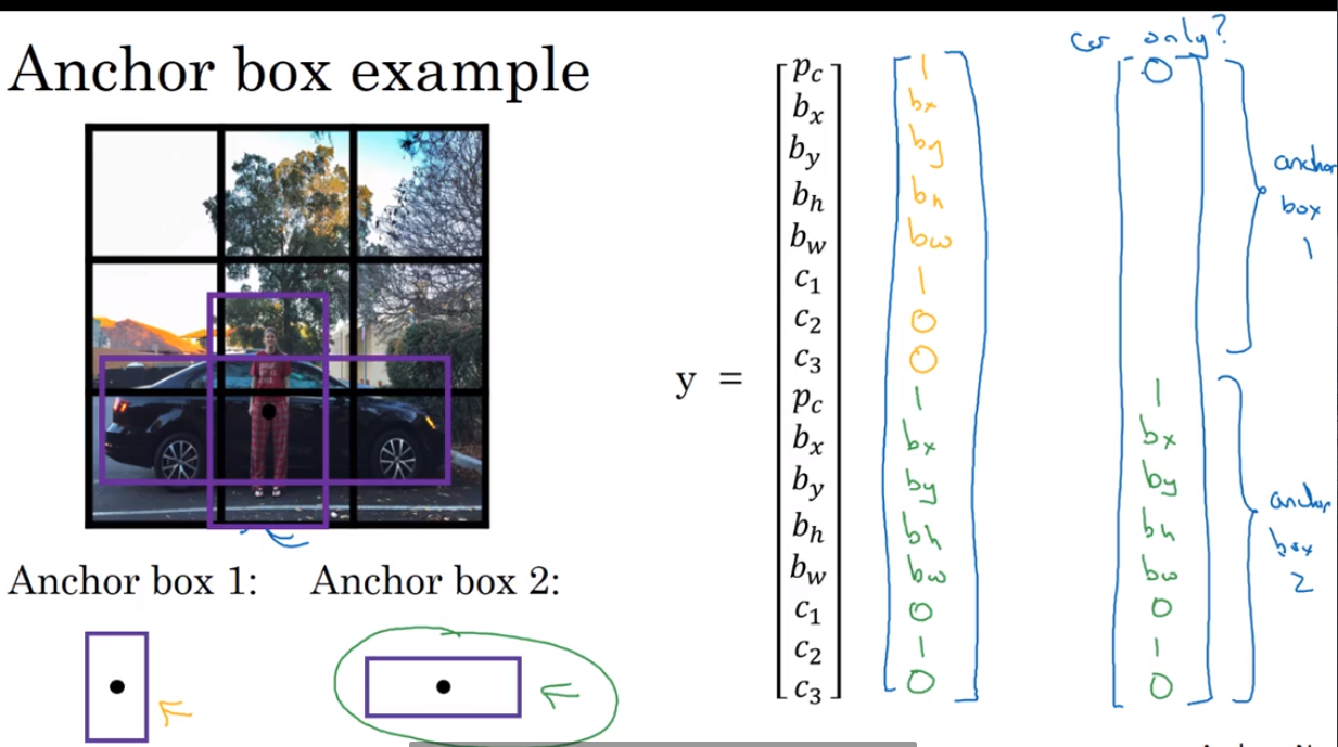
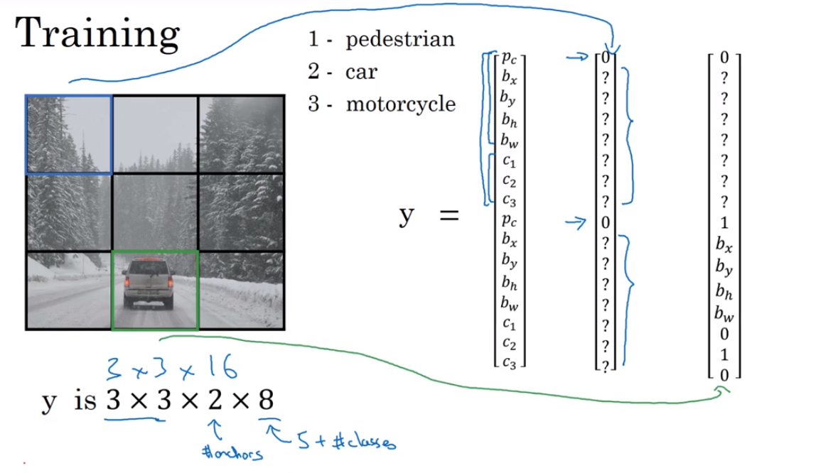
30. Anchor Boxes

Detect multiple objects.

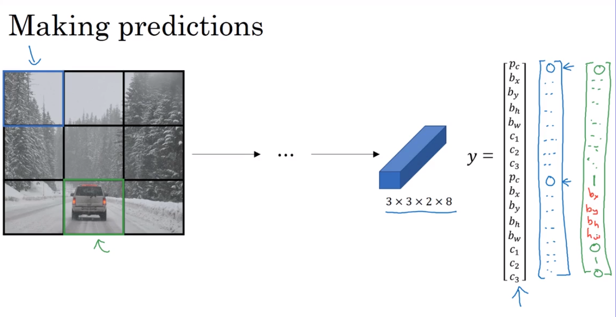
31. YOLO algorithm

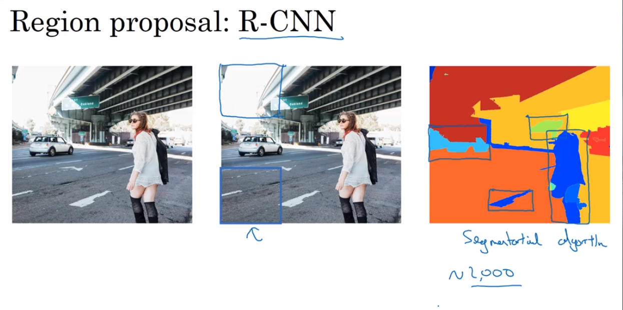
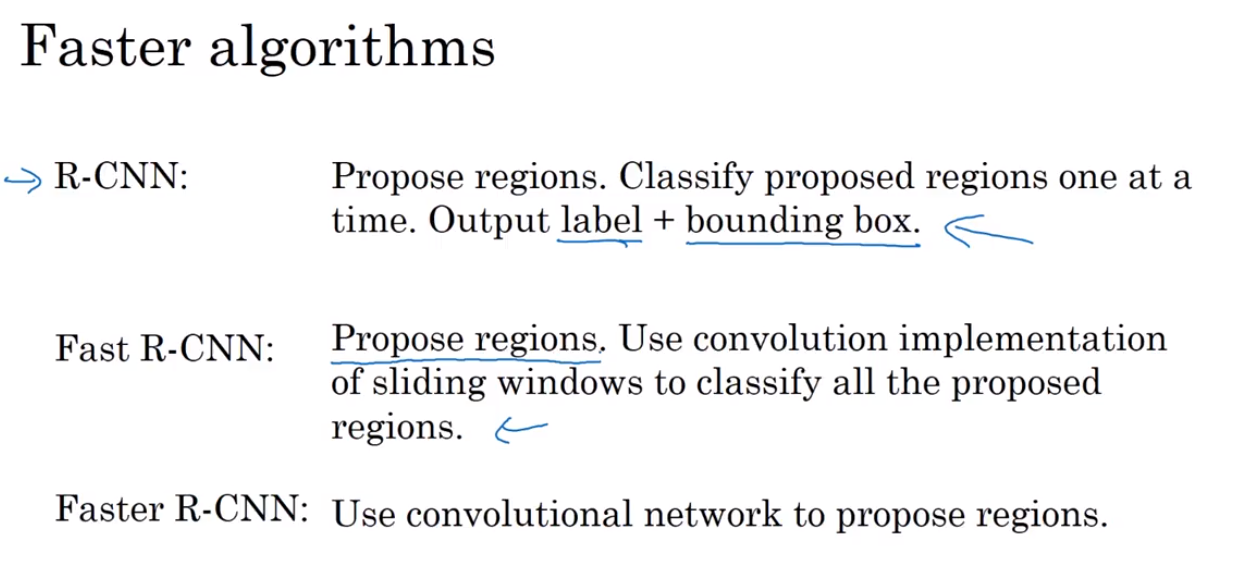
32. Region proposals 候选区域

第四课：视频课33-43

Python 数据分析与应用

基本语法